Executive Summary
Highlights
Science has been one of the foundations of the Montreal Protocol's success. This document highlights advances and updates in the scientific understanding of ozone depletion since the 2018 Scientific Assessment of Ozone Depletion and provides policy-relevant scientific information on current challenges and future policy choices.
- Major Achievements of the Montreal Protocol
- Actions taken under the Montreal Protocol continued to decrease atmospheric abundances of controlled ozone-depleting substances (ODSs) and advance the recovery of the stratospheric ozone layer. The atmospheric abundances of both total tropospheric chlorine and total tropospheric bromine from long-lived ODSs have continued to decline since the 2018 Assessment. New studies support previous Assessments in that the decline in ODS emissions due to compliance with the Montreal Protocol avoids global warming of approximately 0.5-1 °C by mid-century compared to an extreme scenario with an uncontrolled increase in ODSs of 3-3.5% per year.
- Actions taken under the Montreal Protocol continue to contribute to ozone recovery. Recovery of ozone in the upper stratosphere is progressing. Total column ozone (TCO) in the Antarctic continues to recover, notwithstanding substantial interannual variability in the size, strength, and longevity of the ozone hole. Outside of the Antarctic region (from 90°N to 60°S), the limited evidence of TCO recovery since 1996 has low confidence. TCO is expected to return to 1980 values around 2066 in the Antarctic, around 2045 in the Arctic, and around 2040 for the near-global average (60°N-60°S). The assessment of the depletion of TCO in regions around the globe from 1980-1996 remains essentially unchanged since the 2018 Assessment.
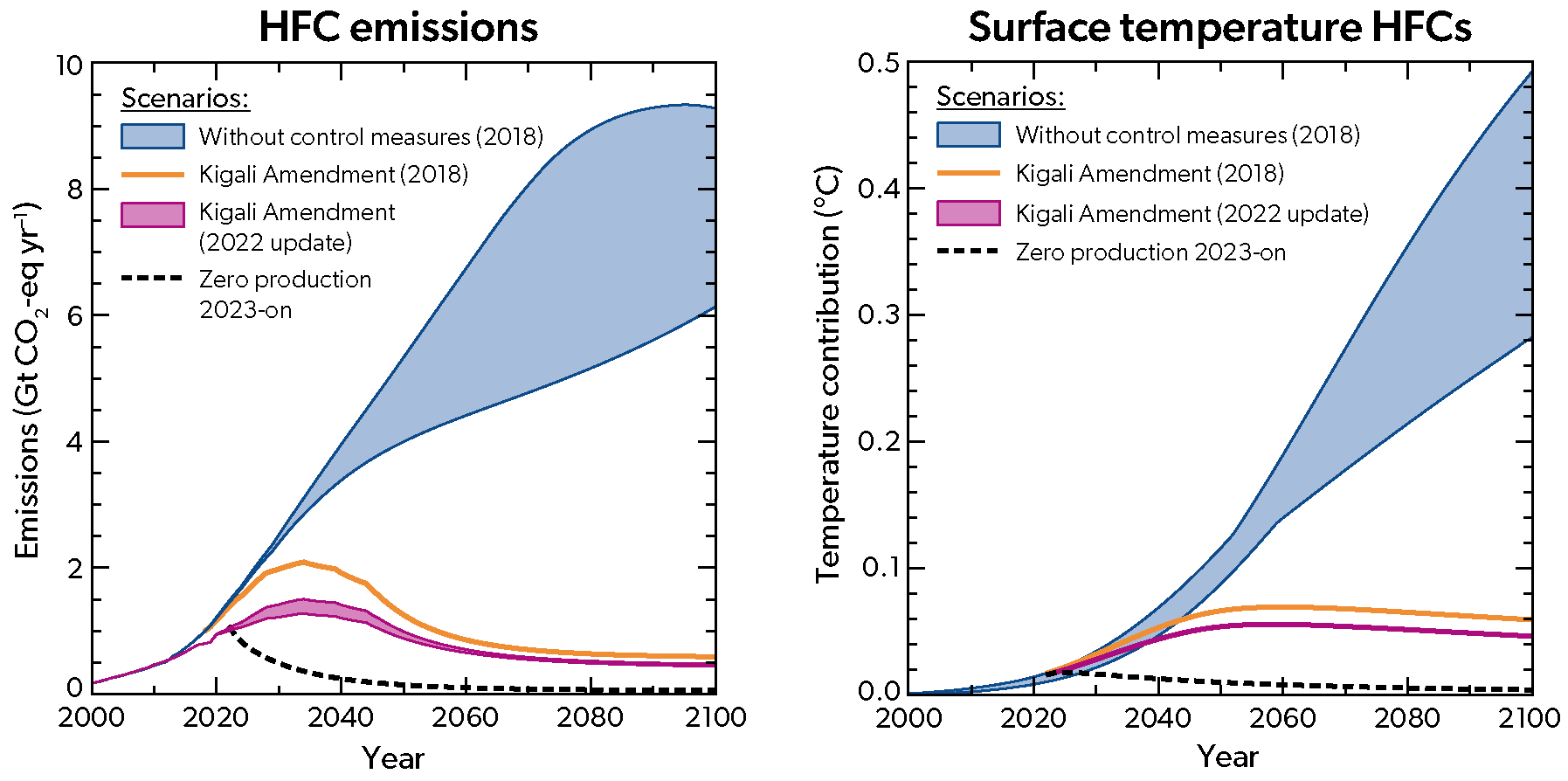
- Compliance with the 2016 Kigali Amendment to the Montreal Protocol, which requires phase down of production and consumption of some hydrofluorocarbons (HFCs), is estimated to avoid 0.3-0.5°C of warming by 2100. This estimate does not include contributions from HFC-23 emissions.
- Current Scientific and Policy Challenges
- The recent identification of unexpected CFC-11 emissions led to scientific investigations and policy responses. Observations and analyses revealed the source region for at least half of these emissions and substantial emissions reductions followed. Regional data suggest some CFC-12 emissions may have been associated with the unreported CFC-11 production. Uncertainties in emissions from banks and gaps in the observing network are too large to determine whether all unexpected emissions have ceased.
- Unexplained emissions have been identified for other ODSs (CFCs-13, 112a, 113a, 114a, 115, and CCl4), as well as HFC-23. Some of these unexplained emissions are likely occurring as leaks of feedstocks or by-products, and the remainder is not understood.
- Outside of the polar regions, observations and models are in agreement that ozone in the upper stratosphere continues to recover. In contrast, ozone in the lower stratosphere has not shown signs of recovery. Models simulate a small recovery in mid-latitude lower-stratospheric ozone in both hemispheres that is not seen in observations. Reconciling this discrepancy is key to ensuring a full understanding of ozone recovery.
- The existing network of atmospheric monitoring stations provides measurements of global surface concentrations of long-lived ODSs and HFCs resulting from anthropogenic emissions. However, gaps in regional atmospheric monitoring limit the scientific community's ability to identify and quantify emissions of controlled substances from many source regions.
- Several space-borne instruments providing vertically resolved, global, measurements of ozone-related atmospheric constituents (e.g., reactive chlorine, water vapor, and long-lived transport tracers) are due to be retired within a few years. Without replacements of these instruments, the ability to monitor and explain changes in the stratospheric ozone layer in the future will be impeded.
- The impact on the ozone layer of stratospheric aerosol injection (SAI), which has been proposed as a possible option to offset global warming, has been assessed following the terms of reference for the 2022 SAP Assessment Report. Important potential consequences, such as deepening of the Antarctic ozone hole and delay in ozone recovery, were identified. Many knowledge gaps and uncertainties prevent a more robust evaluation at this time.
- Heightened concerns about influences on 21st century ozone include impacts of: further increases in nitrous oxide (N2O), methane (CH4), and CO2 concentrations; rapidly expanding ODS and HFC feedstock use and emissions; climate change on TCO in the tropics; extraordinary wildfires and volcanic eruptions; increased frequency of civilian rocket launches and the emissions of a proposed new fleet of supersonic commercial aircraft.
- Future Policy Considerations
- If ODS feedstock emissions as currently estimated were to be eliminated in future years, the return of mid-latitude Equivalent Effective Stratospheric Chlorine (EESC) to 1980 abundances could be advanced by almost 4 years, largely due to reductions in CCl4, and thereby reduce total climate forcing from ODSs.
- Eliminating future emissions of methyl bromide (CH3Br) from quarantine and pre-shipment applications currently allowed by the Montreal Protocol would accelerate the return of mid-latitude EESC to 1980 abundances by two years (as noted in previous Assessments).
- Emissions of anthropogenic very short-lived chlorine substances, dominated by dichloromethane (CH2Cl2), continue to grow and contribute to ozone depletion. If CH2Cl2 emissions continue at their current level, they will continue to deplete approximately 1 DU of annually averaged global TCO. Elimination of these emissions would rapidly reverse this depletion.
- A 3% reduction in anthropogenic N2O emission, averaged over 2023-2070, would lead to an increase in annually averaged global TCO of about 0.5 DU over the same period, and a decrease of about 0.04 Wm-2 in radiative forcing, averaged over 2023-2100.
- Global emissions of long-lived HFC-23, which are largely a byproduct of HCFC-22 production, are as much as eight times larger than expected and are likely to grow unless abatement increases during HCFC-22 production or feedstock use of HCFC-22 decreases.
- The current combined GWP-weighted emissions of CFCs plus HCFCs are comparable to those of HFCs. Reductions in the future emissions of CFCs and HCFCs requires addressing releases from banks and continuing production and use in allowed manufacturing of feedstocks, in by-products, or in unknown uses, depending upon the compound.
Preface
This document contains information upon which the Parties to the Montreal Protocol on Substances that Deplete the Ozone Layer ("The Parties") will base their future decisions regarding protection of the stratospheric ozone layer and climate from the production and consumption of ozone-depleting substances (ODSs) and their replacements.
The Charge to the Assessment Panels
Specifically, Article 6 of the Montreal Protocol on Substances that Deplete the Ozone Layer states:
Beginning in 1990, and at least every four years thereafter, the Parties shall assess the control measures provided for in Article 2 and Articles 2A to 2I on the basis of available scientific, environmental, technical and economic information.
To provide the mechanisms whereby these assessments are conducted, the Montreal Protocol further states:
". . . the Parties shall convene appropriate panels of experts" and "the panels will report their conclusions . . . to the Parties."
To meet this request, the Scientific Assessment Panel (SAP), the Environmental Effects Assessment Panel, and the Technology and Economic Assessment Panel each prepare, every 4 years, major assessments that update the state of understanding in their purviews. These assessments are made available to the Parties in advance of their annual meetings at which they consider amendments and adjustments to the provisions of the Montreal Protocol.
Sequence of Scientific Assessments
The 2022 Assessment is the latest in a series of assessments prepared by the world's leading scientific experts and under the auspices of the Montreal Protocol in coordination with the World Meteorological Organization (WMO) and/or the United Nations Environment Programme (UN Environment). The 2022 Assessment is the tenth in the series of major assessments that have been prepared by the Scientific Assessment Panel as direct input to the Montreal Protocol process. The chronology of the ten scientific assessments of ozone depletion, along with other relevant reports and international policy decisions, are summarized in Table ES-1.
2022 Assessment Terms of Reference
The terms of reference of the 2022 Assessment for the SAP were decided at the 31st Meeting of the Parties to the Montreal Protocol in Rome, Lazio, Italy (4-8 November 2019) in their Decision XXXI/21 (items 1-3 and 5):
1. To request the Scientific Assessment Panel, the Environmental Effects Assessment Panel and the Technology and Economic Assessment Panel to prepare quadrennial assessment reports and submit them to the Secretariat by 31 December 2022 for consideration by the Open-ended Working Group and the Meeting of the Parties in 2023, and to present a synthesis report by 30 April 2023, noting that the panels should continue to exchange information, during the process of developing their respective reports in order to avoid duplication and provide comprehensive information to the parties to the Montreal Protocol;
2. To request the assessment panels to bring to the notice of the parties any significant developments which, in their opinion, deserve such notice, in accordance with decision IV/13;
3. To encourage the assessment panels to closely involve relevant scientists from Article 5 parties with a view to promoting gender and regional balance, to the best of their ability, in producing the reports;
5. That the 2022 report of the Scientific Assessment Panel should include:
- An assessment of the state of the ozone layer and its future evolution;
- An evaluation of global and polar stratospheric ozone, including the Antarctic ozone hole and Arctic winter/ spring ozone depletion and the predicted changes in those phenomena;
- An evaluation of trends in the top-down derived emissions, abundances and fate in the atmosphere of trace gases of relevance to the Montreal Protocol on Substances that Deplete the Ozone Layer, in particular controlled substances and other substances of importance to the ozone layer, which should include a comparison of bottom-up and top-down estimations of such emissions with a view to addressing unidentified emission sources and discrepancies between reported emissions and observed atmospheric concentrations;
- An evaluation of consistency with reported production and consumption of those substances and the likely implications for the state of the ozone layer, including its interaction with the climate system;
- An assessment of the interaction between changes in stratospheric ozone and the climate system, including possible future policy scenarios relating to ozone depletion and climate impacts;
- Early identification and quantification, where possible, of any other issues of importance to the ozone layer and the climate system consistent with the objectives of the Vienna Convention for the Protection of the Ozone Layer and the Montreal Protocol;
- An assessment of information and research related to solar radiation management and its potential effect on the stratospheric ozone layer;
- Relevant information on any newly detected substances that are relevant for the Montreal Protocol.
The Assessment Process
The process of writing the current Assessment started early in 2020. The co-chairs of the Scientific Assessment Panel (SAP) of the Montreal Protocol (David W. Fahey, Paul A. Newman, John A. Pyle, and Bonfils Safari) considered suggestions from the Parties regarding experts from their countries who could participate in the process. A Scientific Steering Committee (SSC), comprising the co-chairs and an ad-hoc international scientific advisory group, was formed to suggest authors and reviewers from the world scientific community and to help craft the Assessment outline. As in previous Assessments, the participants represented experts from the developed and developing world who bring a special perspective to the process and whose involvement in the Assessment contributes to capacity building. The Authors, Contributors, and Reviewers section at the end of this document provides a listing of the approximately 230 scientists from 30 countries who contributed to the preparation and review of the Assessment.
An initial letter was sent to a large number of scientists and policymakers in November 2020 soliciting comments and inputs on a draft outline along with suggestions for authors for the 2022 Assessment. This was followed by revisions to the outline and recruitment of lead authors and co-authors. Revised chapter outlines were developed between February and April 2021 through a series of online meetings of the SSC and lead authors. The chapter writing process produced four drafts between August 2021 and September 2022 aided by a virtual meeting of the author team and SSC in March 2022 and an in-person meeting in July 2022 at WMO Headquarters in Geneva, Switzerland. The first drafts of the chapters were formally peer-reviewed by over 100 expert reviewers. The chapters were revised by the author teams based on the extensive review comments (numbering over 3500). Review editors for each chapter provided oversight of the revision process to ensure that all comments were addressed appropriately.
At a meeting in Geneva, Switzerland, held on 25-29 July 2022, the Executive Summary contained herein was prepared and completed by the 74 attendees of the meeting. These attendees included the steering committee, chapter lead authors, review editors, some chapter co-authors (selected by the chapter leads), reviewers (selected by the review editors), and some leading experts invited by the steering committee. The Executive Summary, initially drafted by the Assessment SSC, was reviewed, revised, and approved line-by-line. The Highlights section was drafted during the meeting to provide a concise summary of the Executive Summary.
The success of the 2022 Assessment depended on the combined efforts and commitment of a large international team of scientific researchers who volunteered their time as lead authors, contributors, reviewers, and review editors and on the skills and dedication of the assessment coordinator and the editorial and production staff, who are listed at the end of this report.
Table ES-1. Chronology of scientific reports and policy decisions related to ozone depletion.
| Year | Policy Decisions | Scientific Reports |
|---|---|---|
| 1981 | The Stratosphere 1981: Theory and Measurements. WMO No. 11. | |
| 1985 | Vienna Convention | Atmospheric Ozone 1985. Three volumes. WMO No. 16. |
| 1987 | Montreal Protocol | |
| 1988 | International Ozone Trends Panel Report 1988. Two volumes. WMO No. 18. | |
| 1989 | Scientific Assessment of Stratospheric Ozone: 1989. Two volumes. WMO No. 20. | |
| 1990 | London Adjustment and Amendment | |
| 1991 | Scientific Assessment of Ozone Depletion: 1991. WMO No. 25. | |
| 1992 | Methyl Bromide: Its Atmospheric Science, Technology, and Economics (Montreal Protocol Assessment Supplement). UNEP (1992) | |
| 1992 | Copenhagen Adjustment and Amendment | |
| 1994 | Scientific Assessment of Ozone Depletion: 1994. WMO No. 37. | |
| 1995 | Vienna Adjustment | |
| 1997 | Montreal Adjustment and Amendment | |
| 1998 | Scientific Assessment of Ozone Depletion: 1998. WMO No. 44. | |
| 1999 | Beijing Adjustment and Amendment | |
| 2002 | Scientific Assessment of Ozone Depletion: 2002. WMO No. 47. | |
| 2006 | Scientific Assessment of Ozone Depletion: 2006. WMO No. 50. | |
| 2007 | Montreal Adjustment | |
| 2010 | Scientific Assessment of Ozone Depletion: 2010. WMO No. 52. | |
| 2014 | Scientific Assessment of Ozone Depletion: 2014. WMO No. 55. | |
| 2016 | Kigali Amendment | |
| 2018 | Scientific Assessment of Ozone Depletion: 2018. WMO No. 58. | |
| 2021 | Report on Unexpected Emissions of CFC-11. WMO No. 1268. | |
| 2022 | Scientific Assessment of Ozone Depletion: 2022. GAW Report No. 278. |
Introduction
The 1985 Vienna Convention for the Protection of the Ozone Layer is an international agreement in which United Nations States recognized the fundamental importance of preventing damage to the stratospheric ozone layer. The 1987 Montreal Protocol on Substances that Deplete the Ozone Layer and its succeeding amendments, adjustments, and decisions were subsequently negotiated to control the consumption and production of anthropogenic ozone-depleting substances (ODSs) and some hydrofluorocarbons (HFCs). The Montreal Protocol Parties base their decisions on scientific, environmental, technical, and economic information that is provided by their technical panels. The Protocol requests quadrennial reports from its Scientific Assessment Panel that update the science of the ozone layer. This Executive Summary (ES) highlights the key findings of the Scientific Assessment of Ozone Depletion: 2022, as put together by an international team of scientists. The key findings of each of the six chapters of the Scientific Assessment have been condensed and formulated to make the ES suitable for a broad audience.
Ozone depletion is caused by human-related emissions of ODSs and the subsequent release of reactive halogen gases, especially chlorine and bromine, in the stratosphere. ODSs include chlorofluorocarbons (CFCs), bromine- containing halons and methyl bromide, hydrochlorofluorocarbons (HCFCs), carbon tetrachloride (CCl4), and methyl chloroform. The substances controlled under the Montreal Protocol are listed in the various annexes to the agreement (CFCs and halons under Annex A and B, HCFCs under Annex C, and methyl bromide under Annex E)2. These ODSs are long-lived (e.g., CFC-12 has a lifetime greater than 100 years) and are also powerful greenhouse gases (GHGs). As a consequence of Montreal Protocol controls, the stratospheric concentrations of anthropogenic chlorine and bromine are declining.
In addition to the longer-lived ODSs, there is a broad class of chlorine- and bromine-containing substances known as very short-lived substances (VSLSs) that are not controlled under the Montreal Protocol and have lifetimes short- er than about 6 months. For example, bromoform (CHBr3) has a lifetime of 24 days, while chloroform (CHCl3) has a lifetime of 149 days. These substances are generally destroyed in the lower atmosphere in chemical reactions. In general, only small fractions of VSLS emissions reach the stratosphere where they contribute to chlorine and bro- mine levels and lead to increased ozone depletion.
The Montreal Protocol's control of ODSs stimulated the development of replacement substances, firstly HCFCs and then HFCs, in a number of industrial sectors. While HFCs have only a minor effect on stratospheric ozone, some HFCs are powerful GHGs. Previous Assessments have shown that HFCs have been increasing rapidly in the atmosphere over the last decade and were projected to increase further as global development continued in the coming decades. The adoption of the 2016 Kigali Amendment to the Montreal Protocol (see Annex F) will phase down the production and consumption of some HFCs and avoid much of the projected global increase and associated climate change.
Observations of atmospheric ozone are made by instruments on the ground and on board balloons, aircraft, and satellites. This network of observations documented the decline of ozone around the globe, with extreme depletions occurring over Antarctica in each spring and occasional large depletions in the Arctic, and they allowed us to report some indications of recovery in stratospheric ozone in the 2014 and 2018 Assessments. The chemical and dynamical processes controlling stratospheric ozone are well understood, with ozone depletion being fundamentally driven by the atmospheric abundances of chlorine and bromine.
Strong declines in the emissions of ODSs starting in the late 1980s lead to a decline in the abundances of chlorine and bromine starting around the turn of the century. As a result, the first indications of ozone recovery are emerging. In addition to ODSs, model simulations demonstrate that stratospheric ozone concentrations are also affected by the chemical and climate effects of greenhouse gases. In particular, increasing concentrations of the GHGs carbon dioxide (CO2) and methane (CH4) during this century will cause global ozone levels to increase beyond the natural level of ozone observed in the 1960s, primarily because of the cooling of the upper stratosphere and a change of the stratospheric circulation. On the other hand, the chemical effect of increasing concentrations of nitrous oxide (N2O), another GHG, will be to deplete stratospheric ozone.
This 2022 Assessment is the tenth in a series that is provided to the Montreal Protocol by its Scientific Assessment Panel. Completely new to this Assessment is Chapter 6, on the potential effects on ozone of the intentional addition of aerosols to the stratosphere, known as stratospheric aerosol injection (SAI). SAI has been proposed as a potential method to reduce climate warming by increasing sunlight reflection; an unintended consequence of SAI is that it could also affect stratospheric temperatures, circulation and ozone production and destruction rates and transport. This new chapter assesses our understanding of these effects based on the SAI strategy and under different climate warming scenarios, as well as identifying sources of uncertainty in these impacts.
In the other six chapters of this Assessment, many of our previous Assessment findings are strengthened and new results are presented. A clear message of the 2022 Assessment is that the Montreal Protocol continues to be effective at reducing the atmospheric abundance of ODSs.
Executive Summary
[1] Abundances and trends in ozone-depleting substances (ODSs)
Our confidence in the achievements of the Montreal Protocol continues to be based on sustained networks of measurements of long-lived source gas abundances covering several decades. These measurements allow the determination of global abundances, their interhemispheric differences and their trends. The data allow us to derive emissions that can be compared with emissions derived from data reported to the UN Environment Programme, when combined with lifetime information and atmospheric modelling.
Changes in tropospheric chlorine and bromine over 2016—2020:
The atmospheric abundances of both tropospheric chlorine (Cl) and bromine (Br), from long-lived Ozone-Depleting Substances (ODSs) controlled under the Montreal Protocol, continued to decline (Figure ES-1). The observed rate of decline in tropospheric chlorine due to substances controlled under the Montreal Protocol was 15.4 ± 4.1 ppt Cl yr-1 (Table ES-2), which is close to the baseline projection from the 2018 Assessment.
Tropospheric chlorine from very short-lived gases, whose sources are mainly anthropogenic and which are not controlled under the Montreal Protocol, increased by 2.1 ± 0.6 ppt Cl yr-1.
The observed rate of decline in tropospheric bromine due to controlled substances was 0.18 ± 0.05 ppt Br yr-1, which is close to the baseline projection from the 2018 Assessment. The majority of this decrease originated from decreases in halon abundances.
Total chlorine and total bromine
Total chlorine entering the stratosphere from controlled and uncontrolled ODSs declined by 420 ± 20 ppt (11.5%) between the 1993 peak (3660 ppt) and 2020 (3240 ppt) (Figure ES-2). This long-term decrease was largely driven by decreasing abundances of CH3CCl3 and CFCs.
HCl is the major chlorine component in the upper stratosphere. Its abundance in this region decreased on average by 0.5 ± 0.2 % yr-1 during 1997-2020. The long-term decrease is consistent with the decline in total chlorine entering the stratosphere.
Total bromine entering the stratosphere from controlled and uncontrolled ODSs declined by 3.2 ± 1.2 ppt (14.5%) between the 1999 peak (22.1 ppt) and 2020 (18.9 ppt). This long-term decrease was largely driven by decreasing abundances of CH3Br and halon-1211.
Total stratospheric bromine, as derived from bromine monoxide (BrO) observations, has decreased by 0.18 ± 0.04 ppt Br yr-1 (0.8% yr-1) since 2003. This decrease is consistent with the decline in total bromine entering in the stratosphere.
CFC-11
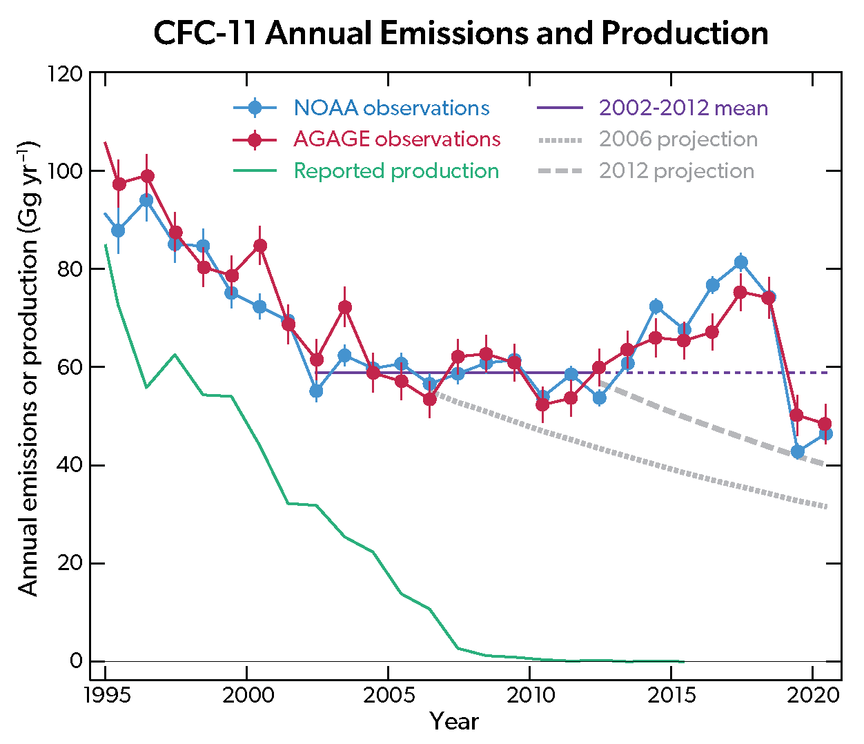
Global CFC-11 emissions declined after 2018, dropping to 45 ± 10 Gg in both 2019 and 2020. This drop suggests the elimination of most of the unexpected emissions occurring in the years after 2012 (Figure ES-3).
A large fraction of the unexpected emissions originated from eastern China. This finding is based on available regional observations from multiple sites. The decline of CFC-11 emissions from eastern China since 2018 explains 60 ± 30% of the observed global emission decrease.
CFC-12
Global CFC-12 abundances continued to decrease during 2016-2020. Estimates of global CFC-12 emissions were 33 ± 21 Gg yr-1 in 2016 and 25 ± 20 Gg yr-1 in 2020.
CFC-12 emissions from eastern China decreased from 3.3 ± 1.4 Gg yr-1 in 2016 to 0.5 ± 0.5 Gg yr-1 in 2019. This decrease is likely associated with the decline in CFC-11 production.
Other CFCs
Global abundances of CFC-13, CFC-112a, CFC-113a, CFC-114a, and CFC-115 increased from 16.0 ± 0.3 ppt in 2016 to a total of 17.2 ± 0.3 ppt ppt Cl in 2020. These changes suggest stable or increasing emissions. Atmospheric observations confirm that eastern Asia is a substantial source region.
Carbon tetrachloride (CCl4)
The atmospheric abundance of CCl4 continued to decrease at slower rates than expected, which could be due to underestimated emissions from feedstock production and usage. Global CCl4 emission estimates based on atmospheric observations are now more accurate than in the last Assessment due to an improved lifetime estimate, and were on average 44 ± 15 Gg yr-1 in both 2016 and 2020.
Emissions of CCl4 in eastern China over the period 2013-2019 show year-to-year variability likely related to CFC-11 production. Emissions increased after 2013, reaching 11.3 ± 1.9 Gg yr-1 in 2016, and decreased to 6.3 ± 1.1 Gg yr-1 in 2019.
Hydrochlorofluorocarbons (HCFCs)
Tropospheric chlorine from HCFCs has continued to increase, reaching 320 ± 3 ppt in 2020. The annual average growth rate of chlorine from HCFCs decreased from 5.9 ± 1.3 ppt yr-1 reported in the 2018 Assessment to 2.5 ± 1.0 ppt yr-1 during 2016-2020.
Global emission estimates of HCFC-22 show evidence of a decline in 2020 after a period of relatively constant emissions. HCFC-142b emissions continued to decline, and HCFC-142b abundances have started to decrease. In contrast, HCFC-141b as well as several low-abundance HCFCs (HCFC-31, HCFC-124, HCFC-133a, and the newly detected HCFC-132b) show stable or increasing emissions.
Halons and methyl bromide (CH3Br)
Bromine from halons has decreased from a peak of 8.5 ± 0.1 ppt in 2006 to 7.3 ± 0.1 in 2020. Halon-1211, halon-2402, and halon-1202 abundances continued to decline between 2016 and 2020. The rate of change of halon-1301 remained indistinguishable from zero. In 2020 it was the most abundant halon in the atmosphere.
Methyl bromide (CH3Br) abundances have varied annually between 6.5 ppt and 6.9 ppt during 2016-2020 with no clear overall trend. Most anthropogenically produced CH3Br has been phased out except for quarantine and pre-shipment (QPS) fumigation, leaving natural emissions as the dominant source. Reported QPS consumption has been relatively stable for more than two decades.
Halogenated very short-lived substances (VSLSs)
Dichloromethane (CH2Cl22), the main component of VSLS chlorine, continued to increase between 2016 and 2020 with a slightly lower growth rate than prior to 2016. This increase primarily results from growing CH2Cl2 emissions in Asia.
Tropospheric chlorine based on measurements of VSLS source gases increased by about 10 ppt between 2016 and 2020. The estimated input of chlorine from VSLSs to the stratosphere also increased by about 10 ppt and amounts to 130 ± 30 ppt in 2020, contributing about 4% of the total chlorine input (Figure ES-2).
Chlorinated VSLSs contribute 4% to the total stratospheric chlorine input in 2020 (Figure ES-2). The VSLSs chlorine input is estimated as 130 ± 30 ppt in 2020 compared to 120 ± 40 ppt in 2016.
Brominated VSLSs, with mainly natural sources, contribute 5 ± 2 ppt to stratospheric bromine and show no long-term changes.
New evidence suggests that iodine from mostly natural sources is entrained into the stratosphere, contributing 0.3 - 0.9 ppt VSLS iodine in particulate or gas-phase form. No observational trend estimates exist.
Other gases that influence stratospheric ozone and climate
Three major greenhouse gases – CH4, N2O, and CO2 – cause changes in stratospheric chemistry and dynamics that can affect O3. An increase in N2O depletes ozone, and increases in CH4 and CO2 tend to increase global stratospheric column ozone. These gases have increased over the industrial era and continue to increase, and are thus additional factors, beyond ODSs, that control stratospheric O3 trends.
Anthropogenic N2O emissions in 2020, when expressed as a CFC-11-equivalent, were more than two times the ODP-weighted emissions from all CFCs in that year, and more than 20% of the CFC emissions in 1987, when the latter were at their peak.
The abundances of many non-ODS, non-HFC, highly fluorinated substances (e.g., SF6, perfluorocarbons, SO2F2, NF3) have continued to increase. While these species do not deplete ozone, they are very strong greenhouse gases with long atmospheric residence times. Total direct radiative forcing due to anthropogenic emissions from these species increased from 0.013 W m-2 in 2016 to 0.014 W m-2 in 2020.
Decarbonization of the fossil fuel industry through a transition to molecular hydrogen (H2) could lead to large increases in atmospheric H2. Estimates from the few existing studies point to relatively small impacts of H2 on future global stratospheric ozone. Global abundances of H2 increased by about 70% since preindustrial times and have varied between 530 and 550 ppb since the late 20th century.
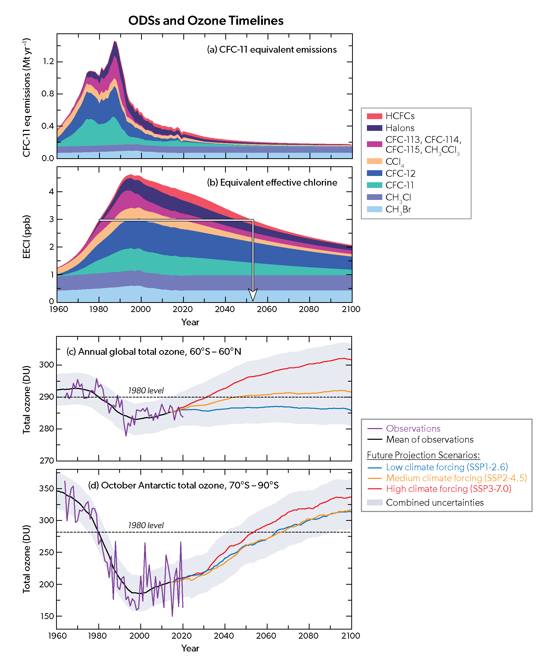
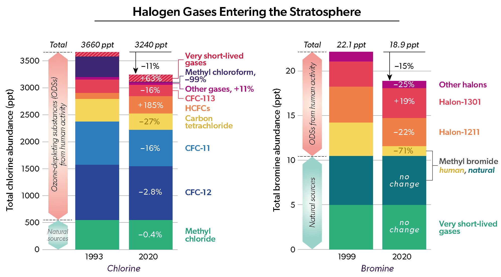
Table ES-2. Contributions of ODSs controlled under the Montreal Protocol to tropospheric chlorine and bromine in 2020, and annual average trends between 2016 and 2020.
| Contribution to tropospheric chlorine and bromine in 20201 (ppt Cl/Br) | Changes in tropospheric chlorine and bromine (in parts per trillion (ppt) (Cl/Br) yr-1) from early-2016 to late-2020 | |
|---|---|---|
| Controlled chlorine substances by group | ||
| chlorofluorocarbons (CFCs) | 1935 | −12.9 ± 2.0 |
| methyl chloroform (CH3CCl3) | 4.2 | −0.90 ± 0.04 |
| carbon tetrachloride (CCl4) | 308 | −3.8 ± 1.0 |
| hydrochlorofluorocarbons (HCFCs) | 319 | 2.5 ± 0.4 |
| halon-1211 | 3.16 | −0.10 ± 0.02 |
| Total Chlorine from controlled substances | 2560 | −15.1 ± 2.4 |
| Controlled bromine substances by group | ||
| halons | 7.3 | −0.11 ± 0.02 |
| methyl bromide (CH3Br)2 | 6.6 | −0.07 ± 0.02 |
| Total bromine from controlled substances | 13.9 | −0.18 (± 0.05) |
1 Values are annual averages.
2 Some anthropogenic uses of CH3Br are exempted from Montreal Protocol controls, and CH3Br has natural sources, which results in a natural background concentration.
[2] Hydrofluorocarbons (HFCs)
Hydrofluorocarbons (HFCs) do not contain ozone-depleting chlorine or bromine. Similar to long-lived CFCs and HCFCs, some HFCs have high global warming potentials. The Kigali Amendment to the Montreal Protocol, which was adopted in 2016 and came into force in 2019, sets schedules for the phase-down of production and consumption of specific HFCs. The radiative forcing due to HFCs is currently small, and the Kigali Amendment was designed to avoid uncontrolled radiative forcing growth in coming decades. HFCs were included as one group within the basket of gases of the 1997 Kyoto Protocol and as a result some countries supply annual emission estimates of HFCs to the United Nations Framework Convention on Climate Change (UNFCCC). The Kigali Amendment initiated additional reporting of production and consumption of HFCs and the emissions of HFC-23. HFC-23 is considered separately primarily because it is emitted to the atmosphere largely as a by-product of HCFC-22 production. This reporting will become more complete as more Parties ratify this Amendment.
Observed HFC abundances and associated emissions
Global atmospheric abundances and emissions of most HFCs are increasing. CO2-equivalent emissions of HFCs derived from observations increased by 18% from 2016 to 2020.
Global HFC emissions derived from atmospheric observations are larger than those reported by Annex I Parties to UNFCCC. The gap between these estimates has grown since the previous Assessment. In 2019, Annex I UNFCCC reporting accounted for approximately one third of the global total emissions derived from atmospheric observations.
It is not possible to attribute a substantial fraction of global HFC emissions to individual countries due to limitations in the global monitoring networks and reporting. Observationally based emission estimates are available for some non-Annex I countries. When these are added to UNFCCC Annex I reports, around 40% of global total CO2-equivalent emissions (excluding HFC-23) remain unexplained.
Global emissions of HFC-23 derived from atmospheric observations increased since the previous Assessment, inconsistent with new information suggesting a substantial rise in abatement independent of Kigali Amendment controls. The estimated global emissions of HFC-23 were 17.2 ± 0.8 kt yr-1 in 2019. This value is substantially higher than the emissions of 2.2 kt yr‑1 in that year derived from activity-based estimates. These activity-based estimates are derived from UNFCCC emission reports, information on production and abatement submitted under the Montreal Protocol and the estimated effect of national regulations.
Observational evidence suggests that changes are occurring in the use of certain HFCs and their replacements, HFOs (hydrofluoroolefins), because of national regulations, market developments, and actions related to the implementation of the Kigali Amendment.
- The 2017 - 2019 CO2-eq. emissions of HFCs are approximately 20% lower than those projected in the scenario without national regulations or the controls of the Kigali Amendment.
- HFOs are increasing in the atmosphere, consistent with their increasing use in place of HFCs. Measurements show that atmospheric background abundances of two HFOs at one central European site have increased by an order of magnitude from 2016 to 2020.
The formation in the atmosphere of trifluoroacetic acid (TFA) is expected to increase in the coming decades due to increased use of HFOs and HCFOs. TFA, a breakdown product of some HFCs, HCFCs, HFOs and HCFOs, is a persistent chemical with potential harmful effects on animals, plants, and humans. The concentration of TFA in rainwater and ocean water is in general significantly below known toxicity limits at present. Potential environmental impacts of TFA require future evaluation due to its persistence.
Projections of HFCs and temperature contributions
Since the previous Assessment, updated projections have been made of HFC emissions assuming adherence to the Kigali Amendment (excluding HFC-23). The projected emissions and the associated radiative forcing and temperature change are smaller than estimated previously. The revised projections are based on extended atmospheric observations from 2014 to 2020, updated UNFCCC national emission inventory reports, updated activity data from Annex I countries, and new consumption data from some non-Annex I countries.
Concerted efforts to improve the energy efficiency of refrigeration and air conditioning equipment could lead to reductions in greenhouse gas emissions of the same order as those from the global implementation of the Kigali Amendment. These estimated benefits of improving energy efficiency are highly dependent on the greenhouse gas emission rate from power generation and the pace of decarbonization in the energy sector.
Following the controls of the Kigali Amendment, HFC emissions (excluding HFC-23) in 2050 are projected to be 0.9-1.0 Gt CO2-eq. yr‑1 in the updated 2022 Kigali Amendment scenario, compared to 4.0-5.3 Gt CO2-eq. yr‑1 in the 2018 scenario without control measures (Figure ES-4). The corresponding radiative forcing in 2050 due to HFCs is 0.09-0.10 W m‑2 with adherence to the Kigali Amendment, compared to 0.22-0.25 W m‑2 without control measures. Annual average surface warming from HFCs is expected to be 0.04°C in 2100 under the updated 2022 Kigali Amendment scenario, compared to 0.3-0.5 °C without control measures.
Emissions of HFC-23 are expected to grow in the coming decades unless abatement during HCFC-22 production is increased. This growth is based on an anticipated continued increase in HCFC-22 production, primarily for feedstock use, which is allowed under the Montreal Protocol.
[3] Stratospheric ozone
The Montreal Protocol and its Amendments and Adjustments have been effective in decreasing the abundance of ODSs in the atmosphere. The clearest signs of corresponding ozone recovery are seen in the upper stratosphere and in the Antarctic lower stratosphere in spring. ODS-related ozone recovery is difficult to detect in other regions due to large natural variability and confounding factors, such as climate change and changes in tropospheric ozone. In the Arctic, for example, severe ozone loss occurs only under cold stratospheric conditions (e.g., in spring 2011 and most recently in spring 2020). An Arctic ozone trend is difficult to detect given the much larger variability than in the Antarctic. Episodic volcanic eruptions and, recently, also intense wildfires can increase stratospheric aerosol substantially and hence have the potential to perturb stratospheric ozone. The effects of the Australian wildfires of 2019/2020 and of the large Hunga Tonga-Hunga Ha'apai volcanic eruption in 2022 on ozone are not assessed here and are an area of active research. Ozone in the tropical lower stratosphere shows little response to changes in ODSs, because halogen-driven ozone depletion is comparatively small in this region.
Antarctic and Arctic ozone
Recovery of Antarctic stratospheric ozone continues to progress. New results since WMO (2018) support the findings reported at that time that the Antarctic ozone hole has generally diminished in size and depth since the year 2000. New analyses provide additional evidence that September is the period when stratospheric ozone over Antarctica shows the largest sensitivity to decreasing ODSs, and when Antarctic ozone recovery rates are the strongest and the most statistically significant.
Antarctic ozone holes observed between 2019 and 2021 exhibited substantial variability in size, strength, and longevity. This behaviour is largely dynamically driven, is consistent with our understanding, and does not challenge the evidence for the emergence of recovery. The 2019 ozone hole was the smallest since 2002. In contrast, both 2020 and 2021 had relatively large and long-lasting late-spring ozone holes.
In the Arctic, observed trends in ozone remain small compared to the large year-to-year variability. This precludes the identification of a statistically significant trend in Arctic ozone over the 2000-2021 period.
Arctic total ozone reached exceptionally low values in spring 2020. A very stable, cold, and long-lived stratospheric polar vortex enabled halogen-catalyzed chemical ozone loss that exceeded the previous record-breaking loss observed in spring 2011. The strong vortex also inhibited dynamical replenishment of polar ozone. The evolution of high-latitude ozone in 2020 is successfully reproduced by model simulations, further substantiating our understanding of polar ozone chemistry.
Global ozone
Changes to date in total column ozone
Aggregated ground- and space-based observations indicate an increase of 0.3% decade-1 (with a 2-sigma uncertainty of at least ±0.3% decade-1) in near-global (60°S-60°N) total column ozone over the 1996-2020 period. This trend is consistent with model simulations and our scientific understanding of the processes controlling ozone. Over the same period, trends over broad latitude bands are as follows:
- Southern Hemisphere mid-latitude (35°S-60°S), total column ozone has increased (0.8 ± 0.7% decade-1).
- Northern Hemisphere mid-latitudes (35°N-60°N), total column ozone trends are negligible (0.0 ± 0.7% decade-1).
- Tropical (20°S-20°N) total column ozone shows no clear trend (0.2 ± 0.3% decade-1), likely because lower stratospheric ozone is decreasing while tropospheric ozone is increasing, both unrelated to changes in ODSs.
Present day (2017-2020) total column ozone as measured from space-based and ground-based observations remains lower than the 1964-1980 average, by
- about 2% for the near global average (60°S-60°N)
- about 4% in the Northern Hemisphere mid latitudes (35°N-60°N)
- about 5% in the Southern Hemisphere mid latitudes (35°S-60°S)
- about 1% in the tropics (20°S-20°N).
The latitudinal pattern of these total column ozone trends is largely consistent with our scientific understanding and is reproduced in the latest set of chemistry-climate models.
Within uncertainties associated with natural variability and instrumental accuracy, these values are essentially the same as given in the previous Assessment for the 2014-2017 average.
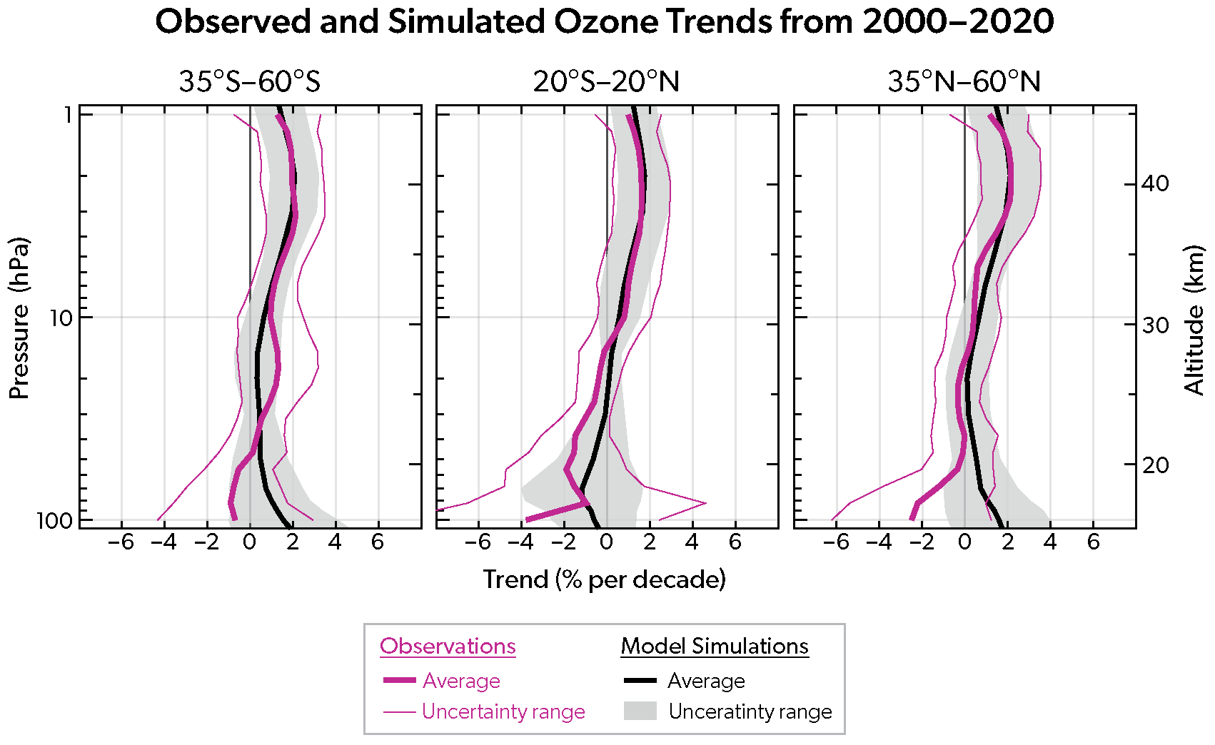
Changes to date in vertically resolved ozone
Vertically resolved trends are very similar to those given in the last Assessment (Figure ES-5). With longer records and updates to merged datasets, uncertainties have been reduced.
Measurements show unambiguous increases in upper stratospheric ozone for 2000-2020 outside of the polar regions. Positive trends have a range of 1.5-2.2% decade-1 at mid-latitudes in both the Northern and Southern Hemispheres and 1.1-1.6% decade-1 in the tropics.
Upper stratospheric ozone increases are due to a combination of decreases in ozone depleting substances and decreases in stratospheric temperature driven by increases in CO2. New model simulations reaffirm this finding from the 2018 Assessment.
There are multiple lines of evidence from both observations and models for a small though uncertain decrease (1-2% decade-1, with uncertainty up to ±5% decade-1) in tropical lower stratospheric ozone over 2000-2020. This decrease is consistent with climate change-driven acceleration of the large-scale circulation and has a small impact on total column ozone. Chemical ozone loss from chlorine and bromine is comparatively minor in the tropical lower stratosphere.
Observations suggest small decreases in lower stratospheric ozone in the mid-latitudes of both hemispheres for 2000-2020, while chemistry climate model simulations suggest small increases. Ozone in mid-latitudes has large year-to-year variability; thus trends have large uncertainties, and they are not robust across all datasets and models. The observed decrease is more evident in the Northern Hemisphere.
Outside of polar regions, attribution of total column ozone trends during the period of slow ODS decline requires knowledge of changes in ozone in both the troposphere and stratosphere. For instance, there is evidence that the lack of a change in total column ozone in the tropics reflects an increase in tropospheric ozone that compensates for the ozone decrease in the tropical lower stratosphere.
Future ozone changes
As reported in the last Assessment, the key drivers of future stratospheric ozone levels continue to be declining ODSs coupled with CO2-driven cooling in the upper stratosphere and a strengthening of the Brewer-Dobson circulation. Total column ozone will also be affected by changes in the tropospheric ozone burden.
New estimates for the year of return of total column ozone outside of polar regions to 1980 values are broadly consistent with the last Assessment. Also similar to the 2018 Assessment, these modelled return dates vary considerably depending on the assumed future greenhouse gas scenario. Total column ozone returns to 1980 values sooner for scenarios that assume larger emissions of greenhouse gases than scenarios with smaller greenhouse gas emissions. Broadly, the return dates for a middle-of-the-road (SSP2-4.5) scenario are consistent with previous Assessments:
- around 2040 for near global mean (60°S-60°N) annually averaged column ozone;
- around 2045 for Southern Hemisphere (60°S-35°S) annually averaged column ozone; and
- around 2035 for Northern Hemisphere (35°N-60°N) annually averaged column ozone.
For scenarios that assume strong reductions in the emission of tropospheric ozone precursors, the resulting reductions in tropospheric ozone can be important for total column ozone trends. Under such scenarios, total column ozone in the tropics is projected to remain below the 1980 values until at least 2100. As discussed in the last Assessment, tropical total column ozone under high greenhouse gas (GHG) scenarios will be below 1980 values at 2100 due to circulation-driven changes affecting lower stratospheric ozone.
The Antarctic ozone hole is expected to gradually close, with springtime total column ozone returning to 1980 values shortly after mid-century (about 2065). Updated chemistry-climate model projections suggest that ozone hole recovery may depend on the future climate change scenario, with projections of return around 2050 for the low climate change mitigation scenarios. This sensitivity of Antarctic recovery to climate change scenario differs from the findings in previous Assessments and may be due to the use of a smaller number of updated models, as well as the models being forced with different evolutions of GHGs.
Arctic springtime total ozone is expected to return to 1980 values slightly before mid-century (about 2045). Substantial Arctic ozone loss will occur in cold winters/springs as long as ODS concentrations are well above natural levels. While dynamical changes associated with increasing GHGs lead to an earlier recovery of Arctic ozone, increasing stratospheric water vapor abundances and CO2-driven cooling of the lower stratosphere may increase the potential for the formation of polar stratospheric clouds in dynamically undisturbed Arctic winters, leading to ozone loss.
The unreported production of CFC-11 over 2012-2019 is estimated to delay polar ozone return to 1980 values by up to 3 years. For global total column ozone, the delay is about 1 year.
Exceptional events can temporarily perturb chemical and dynamical processes that affect stratospheric ozone amounts. Since the last Assessment, these include the 2019/2020 wildfires in Australia, the eruption of the Hunga Tonga-Hunga Ha'apai volcano, and disruptions to the quasi-biennial oscillation of the tropical winds. In particular, intense wildfires have become more frequent. Their potential impacts on the stratosphere are not yet well quantified and are a subject of active research.
The impending loss of vertically resolved, global spaceborne measurements of ozone-related atmospheric constituents (e.g., reactive chlorine, water vapour, and long-lived transport tracers) will impede the ability to monitor and explain changes in the stratospheric ozone layer in the future.
[4] Ozone change and its influence on climate
Stratospheric ozone has a wide-ranging influence on the Earth system. Antarctic ozone depletion caused expansion of the tropics and a poleward shift of the jet stream and storm tracks in the Southern Hemisphere that lead to pronounced changes in summertime surface climate, as summarized in the previous Assessments. Continuing ozone recovery and increases in atmospheric greenhouse gas (GHG) concentrations will be key drivers of future Southern Hemisphere climate changes. The relative importance of ozone recovery for future Southern Hemisphere climate will depend on the magnitude and rate of atmospheric GHG concentration changes.
Evolution of stratospheric climate
The estimated rate of long-term cooling in the global middle and upper stratosphere (0.6 K decade-1) is similar to previous Assessments. The evolution of stratospheric temperatures continues to follow the behavior expected from the well understood effects of natural and anthropogenic forcings. The long-term trends are primarily driven by changing CO2 and stratospheric ozone. Global temperature in the lower stratosphere has been near constant since the late 1990s.
In the future, increasing GHGs and the effects of ozone recovery would have opposing effects on stratospheric temperature and circulation. For a moderate GHG emission scenario (RCP6.0), stratospheric cooling and the acceleration of the global stratospheric transport circulation (the Brewer Dobson Circulation) driven by increasing GHGs dominate over opposing effects from ozone recovery. Under both moderate (RCP4.5/SSP2-4.5) and high emission (RCP8.5/SSP5-8.5) scenarios, the delayed breakdown of the austral springtime polar vortex that was driven by ozone depletion in the late 20th century will persist due to the effect of increasing GHGs.
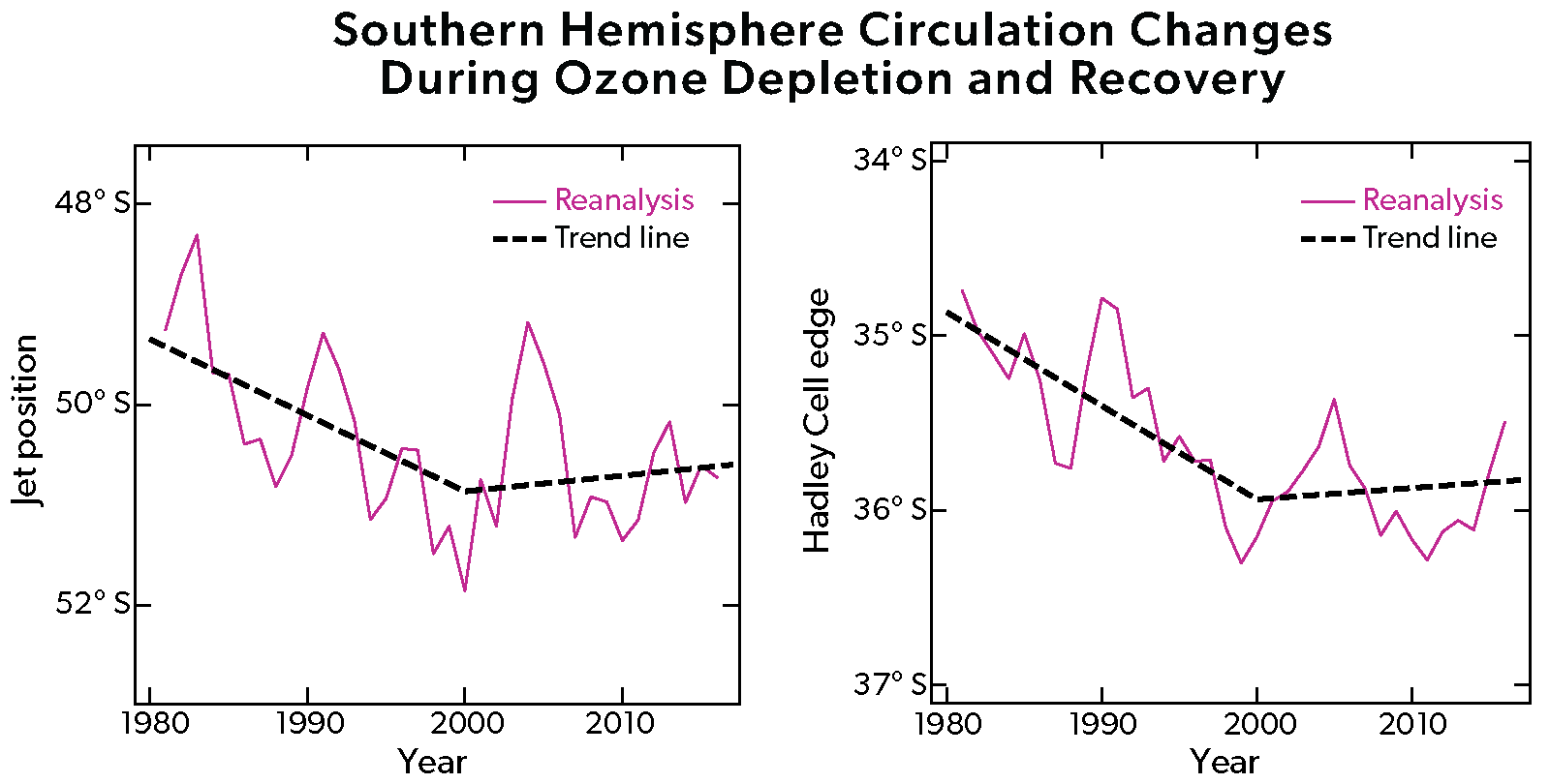
Influence on tropospheric and surface climate
New evidence suggests that ozone recovery has caused changes in the observed trends of the Southern Hemisphere atmospheric circulation between the ozone depletion and recovery periods. Model simulations support the attribution of these changes to ozone recovery. These results provide evidence that Southern Hemisphere circulation trends have responded to the recovery of Antarctic ozone due to the Montreal Protocol (see Figure ES-6).
While there are no detectable surface impacts of long-term Arctic ozone changes, new evidence shows that for individual years low springtime Arctic ozone can amplify existing stratospheric circulation anomalies and their influence on tropospheric circulation and surface climate.
Influence on the Southern Hemisphere ocean & cryosphere
New evidence confirms that ozone depletion is unlikely to have driven the observed high-latitude sea-surface temperature cooling and changes in Antarctic sea ice since 1979. There is no robust link between ozone depletion and net Southern Ocean carbon uptake, which exhibits large decadal variations.
Radiative forcing from past ODS, HFC & stratospheric ozone changes
The calculated total direct radiative forcing due to CFCs, HCFCs, halons, CCl4 and CH3CCl3 decreased by 0.006 W m-2 since 2016 and was 0.337 W m-2 in 2020. This forcing is approximately 16% of the radiative forcing of CO2. CO2-equivalent emissions (in Gt CO2-eq yr-1) in 2020 were, for species where estimates are available, 0.7 ± 0.4 for CFCs, 0.7 ± 0.1 for HCFCs, 0.09 ± 0.03 for CCl4 and CH3CCl3 combined, and 0.02 ± 0.001 for halons.
The best estimate of radiative forcing from stratospheric ozone changes over 1850-2011 is -0.02 W m-2, with an uncertainty of ± 0.13 W m-2. Hence, the combined radiative forcing from ODSs and historical stratospheric ozone changes is positive (around 0.3 W m-2), consistent with previous Assessments.
Radiative forcing from measured HFCs continues to increase. The radiative forcing due to the HFCs reached 0.044 ± 0.006 W m-2 in 2020, an increase of around one-third since 2016. The most important contributor to HFC radiative forcing was HFC-134a (44%), and HFC-125 (18%) overtook HFC-23 (15%) as the second largest contributor. Together, the HFCs represent approximately 2% of the radiative forcing of CO2. Total CO2-equivalent emissions in 2020 were 1.22 ± 0.05 Gt CO2-eq yr-1.
Climate impacts of the control of ODSs by the Montreal Protocol
New studies support previous Assessments that the decline in ODS emissions due to the implementation of the Montreal Protocol avoids an additional global warming of approximately 0.5-1 K by mid-century compared to an extreme scenario with an uncontrolled increase in ODSs of 3-3.5% per year and the resulting changes in ozone. New evidence suggests an additional avoided warming by mid-century due to prevention of UV radiation damage to the terrestrial carbon sink, as such damage would cause additional CO2 to remain in the atmosphere.
[5] Stratospheric aerosol injection & potential impacts on ozone
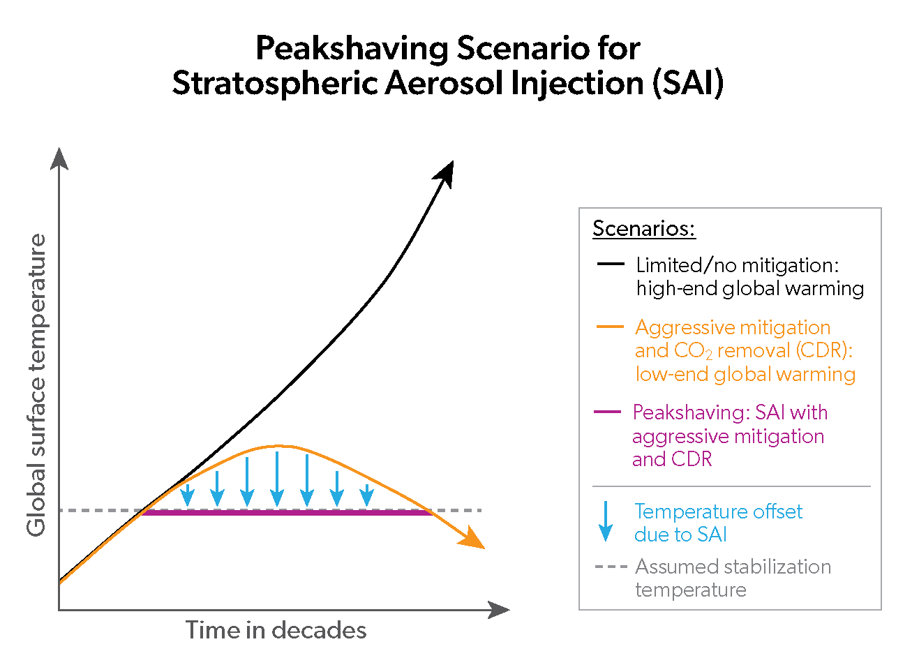
Global warming has now reached approximately 1.2°C above pre-industrial levels. Climate model scenarios considered by IPCC (2021) indicate continued future warming in the next few decades even with ambitious mitigation and decarbonization, leading to further climate impacts. Stratospheric Aerosol Injection (SAI) has the potential to limit the rise in global surface temperatures by increasing the concentrations of particles in the stratosphere. These particles reflect a fraction of sunlight back to space, in a process similar to that evident after large volcanic eruptions. However, SAI comes with significant risks and can cause unintended consequences. The 2022 Assessment is the first to dedicate a chapter to assess the potential impacts on stratospheric ozone in possible SAI scenarios in the coming decades based on the limited number of model simulations that have been performed to date.
Stratospheric Aerosol Injection (SAI) has the potential to reduce global mean temperatures. However, SAI cannot fully offset the wide-spread effects of global warming and produces unintended consequences, including effects on ozone. Details of these effects depend on the specifics of the SAI scenario and SAI injection strategy</p>
- In different SAI scenarios, the modeled effects of SAI on future ozone depend on the specific details of future climate change, and on the amount, timing and duration of SAI applied. Offsetting an ever-increasing global warming with an ever-increasing SAI ("strong SAI") has been shown to lead to increasing environmental risks.
- In a world with limited mitigation of greenhouse gas emissions, global mean temperatures continue to increase significantly in the future (Figure ES-7, black line). This future warming would be reduced by aggressive decarbonisation (orange line). A SAI peakshaving scenario offsets the overshoot of surface temperature above a certain threshold until greenhouse gases have been reduced (purple line).
- Different SAI strategies such as the altitude and latitude of injection, and type of material, have been developed to mitigate some of the unintended climate impacts of SAI. In modelling studies, the principal injected material is sulfur. Different strategies would have different effects on stratospheric ozone.
Model simulations of SAI reveal large differences in surface cooling per unit sulfur injected, which are attributed to differences in representing key processes. Explosive volcanic eruptions serve as natural analogues to aid evaluation of these models.
- Very few Earth System Models resolve complex stratospheric processes, including detailed aerosol microphysics coupled with chemistry, radiation and dynamics. In addition, the sparsity of current existing model simulations limits the confidence in the quantification of many impacts.
- Injection rates vary between 8 and 16 Mt of SO2 per year to cool the Earth by 1°C (an injection amount approximately equivalent to that of the Mt Pinatubo eruption in 1991), based on simulations with seven Earth System Models.
- Explosive volcanic eruptions sporadically emit millions of tonnes of sulphur dioxide (SO2) into the stratosphere and provide useful, albeit imperfect, natural analogues for evaluating the global models used to conduct SAI simulations.
The net effects of large-scale SAI on stratospheric ozone are mainly driven by i) increases in aerosol surface area, ii) stratospheric halogen and nitrogen concentrations, and iii) aerosol-induced heating of the stratosphere, which change both stratospheric ozone chemistry and stratospheric dynamics. These simulated changes are strongly model dependent.
- Enhanced stratospheric sulfate aerosol increases stratospheric heterogeneous chemical reaction rates, leading to enhanced or depleted stratospheric ozone depending on altitude, latitude and season. Details depend on the SAI-induced aerosol surface-area distribution, the current stratospheric halogen and nitrous oxide concentrations, and SAI-induced changes in stratospheric water vapour.
- Increased sulfate aerosols in SAI scenarios heat the lower tropical stratosphere by 4.6 ± 2.7 °C per 1°C surface cooling based on results from different models and injection scenarios. Resulting changes in stratospheric composition and transport depend on the details of the injection strategy and are strongly model dependent.
Additional ozone depletion due to SAI is simulated in spring over Antarctica, with magnitudes dependent on the injection rate and timing. Simulations of strong SAI show an increase in total column ozone (TCO) in mid-latitudes (40-60°N) in the winter Northern Hemisphere.
- For October over Antarctica, SAI simulations that achieve a global mean surface cooling of 0.5°C in the first 20 years, show a reduction of TCO of around 58 ± 20 DU, assuming 2020-2040 halogen conditions. This reduction brings TCO values close to the observed minimum in the 1990s. Less ozone loss would be expected for a later SAI start date when halogen concentrations are projected to be lower.
- Beyond the first 20 years, the continued application of strong SAI, to offset almost 5°C of warming by 2100, reduces Antarctic ozone in October by similar amounts (55 ± 20 DU) throughout the 21st century despite declining abundances of ozone-depleting substances (ODS). In this case, ozone-hole recovery from ODSs is delayed by between 25 and 50 years. A peakshaving scenario potentially leads to less ozone depletion.
- Under stronger SAI scenarios, ozone is significantly enhanced in NH mid-latitudes in winter owing to stratospheric heating from injected sulfur, which leads to increased equator to poleward transport of ozone.
- Ozone loss within the Arctic polar vortex has not yet been robustly quantified for SAI.
The injection of aerosols other than sulfate is expected to change the effects on ozone via associated changes in heterogeneous chemistry, dynamics and transport. Aerosol types that are more chemically inert and absorb less solar radiation may reduce chemical and dynamical impacts on stratospheric ozone respectively. However, the laboratory studies and climate model simulations sufficient to quantify these effects have yet to be performed.
[6] Policy-relevant scenarios and information
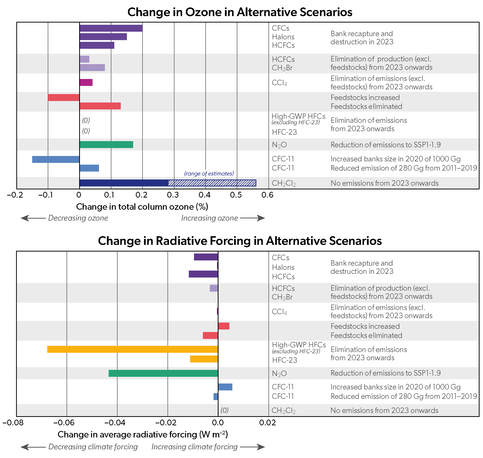
Changes in total column ozone and in average radiative forcing in response to various control measures using alternative scenarios and bounding test cases are shown in Figure ES-8. The baseline scenario used here assumes full compliance with the Montreal Protocol. The hypothetical alternative scenarios assessed here include the elimination of banks, production, and emissions of gases that are both controlled and uncontrolled by the Montreal Protocol and are intended to demonstrate the impacts on climate and ozone relevant to policy actions.
The unexpected emissions of CFC-11 over 2012-2019 have led to a delay in the return of mid-latitude EESC to 1980 abundances by about 1 year. The reduction in emissions since 2018, based on global and regional observations, have prevented a longer delay.
The CFC-11 production that led to these observed unexpected emissions has most likely increased global banks. Assuming these emissions were associated with the production of insulating foams, it is estimated that they account for 25% to 45% of the unreported production. This suggests a potential increase in the CFC-11 bank of 146-1320 kt from unreported production between 2012 and 2019. For reference, a 1000 kt increase in the 2020 bank would further delay the return of mid-latitude EESC to 1980 levels by almost 4 years (Figure ES-8).
If it were possible to eliminate all future long-lived anthropogenic ODS emissions in 2023, this would bring forward the return of mid-latitude EESC to 1980 abundances by about 16 years and increase the average of global stratospheric ozone in the period 2023-2070 by about 2 DU. This provides an upper limit for the reduction of EESC through control measures. These emissions are dominated by the release from current banks, with additional contributions from controlled future production and consumption of ODSs, production for feedstock use, and quarantine and pre-shipment uses of CH3Br.
The projected return of mid-latitude EESC is delayed by 6 years compared with the previous Assessment due mostly to larger assessed banks in the current baseline scenario. The larger bank estimates primarily arise from the use of a new modelling approach to assess the banks.
Total production of controlled substances for feedstock use is increasing. If all future feedstock-related emissions were eliminated, this would bring forward the return of mid-latitude EESC to 1980 levels by almost 4 years when compared to the baseline scenario. Reported feedstock production has increased by 75% by mass over the last decade. Assuming that the fraction of emissions related to feedstock production has not changed, emissions have increased accordingly. Additionally, feedstock usage has led to the emissions of a range of ODS by-products and intermediates.
The CCl4 emissions from feedstock production and use currently dominate the ODS influence on ozone from all feedstocks. The elimination of these CCl4 emissions accomplishes much of the projected 4-year accelerated return in EESC noted above. This usage of CCl4 is expected to continue increasing primarily because of its application in the growing production of HFOs, and could roughly double CCl4 abundances in 2100 compared to the baseline scenario.
If future emissions of methyl bromide (CH3Br) from quarantine and pre-shipment (QPS) applications could be eliminated, this would accelerate the return of mid-latitude EESC by about 2 years. Production for QPS use has remained nearly unchanged over the last two decades. It now constitutes almost 99% of the reported production of CH3Br, with critical use exemptions (CUEs) making up the remaining reported production. The importance of QPS CH3Br has been noted in previous Assessments.
Abundances of several gases not controlled by the Montreal Protocol have been increasing due primarily to anthropogenic emissions and have direct effects on stratospheric ozone, for example dichloromethane (CH2Cl2) and N2O.
Emissions of CH2Cl2, the dominant anthropogenic VSLS chlorine gas, continue to increase and augment ozone-depleting chlorine in the atmosphere. Future projections are uncertain due to the highly variable emissions over the past few years. If CH2Cl2 emissions continue at their current level, they will continue to deplete approximately 1 DU of global, annual average ozone. Elimination of these emissions would rapidly reverse this depletion. (Figure ES-8).
A 3% reduction in anthropogenic N2O emissions, averaged over 2023-2070, leads to an increase in global ozone of about 0.5 DU averaged over the same period, and a decrease of about 0.04 W m-2 in radiative forcing, averaged over 2023-2100 (Figure ES-8). This reduction is the amount obtained when comparing the baseline N2O scenario (SSP2-4.5) to the strongest N2O mitigation scenario of the SSPs (SSP1-1.9).
Scientific Summaries of the Chapters
Chapter 1: Update on Ozone-Depleting Substances (ODSs) and other Gases of Interest to the Montreal Protocol
This chapter concerns atmospheric changes in ozone-depleting substances (ODSs), such as chlorofluorocarbons (CFCs), halons, chlorinated solvents (e.g., carbon tetrachloride [CCl4] and methyl chloroform [CH3CCl3]) and hydrochlorofluorocarbons (HCFCs), which are controlled under the Montreal Protocol. Furthermore, the chapter updates information about ODSs not controlled under the Protocol, such as methyl chloride (CH3Cl) and very short-lived substances (VSLSs). In addition to depleting stratospheric ozone, many ODSs are potent greenhouse gases.
Mole fractions of ODSs and other species are primarily measured close to the surface by global or regional monitoring networks. The surface data can be used to approximate a mole fraction representative of the global or hemispheric tropospheric abundance. Changes in the tropospheric abundance of an ODS result from a difference between the rate of emissions into the atmosphere and the rate of removal from it.
The total amount of chlorine and bromine from ODSs that were controlled under the original Montreal Protocol is continuing to decline, as the overall emissions are smaller than the rate at which these ODSs are destroyed. Abundances of many of the first-stage replacement compounds, HCFCs, are now increasing very slowly or not at all.
Tropospheric chlorine (Cl)
Total tropospheric chlorine is a metric used to quantify the combined globally averaged abundance of chlorine in the troposphere due to the major chlorine-containing ODSs. The contribution of each ODS to total tropospheric chlorine is the product of its global mean tropospheric mole fraction and the number of chlorine atoms it contains.
Total tropospheric chlorine from ODSs continued to decrease between 2016 and 2020. Total tropospheric chlorine in 2020 was 3,220 ppt (where ppt refers to parts per trillion as a dry air mole fraction), about 1.8% lower than in 2016 and 12% lower than its peak value in 1993. Of the 2020 total, CFCs accounted for about 60%, CH3Cl for about 17%, and CCl4 and HCFCs each for about 10%. The contribution from CH3CCl3 has now decreased to 0.1%. Very short-lived source gases (VSL SGs), as measured in the lower troposphere, contributed approximately 3.5%.
- During the period 2016-2020, the observed rate of decline in tropospheric chlorine due to controlled substances was 15.1 ± 2.45 ppt Cl yr−1, which is larger than during the 2012-2016 period (12.8 ± 0.8 ppt Cl yr−1). This rate of decrease was close to the projections in the previous Assessment. The net rate of change was the result of a slightly slower than projected decrease in CFCs and a slower HCFC increase than in the 2018 A1 projection scenario.
- When substances not controlled under the Montreal Protocol are also included, the overall decrease in tropospheric chlorine was 15.1 ± 3.6 ppt Cl yr−1 during 2016-2020. This is larger than the rate of decline during the 2012-2016 period (3.6 ± 4.7 ppt Cl yr−1) and comparable to the rate of decline in controlled substances. Changes in the predominantly anthropogenic dichloromethane (CH2Cl2) and the largely natural CH3Cl largely canceled each other out, resulting in almost no net change in Cl from uncontrolled substances during this period.
Starting around 2018, the rate at which the CFC-11 mole fraction was declining in the atmosphere accelerated again, following a slowdown since 2013. These recent changes are largely due to a decrease in emissions originating mostly from northeastern China. Assuming no impact from changes in atmospheric circulation, global emissions increased from about 57 Gg yr-1 (= kt yr-1) in 2012 to around 78 Gg yr-1 in 2017; after 2018, they then decreased, to approximately 47 Gg yr-1 in 2020. Emissions from northeastern China explain 60 ± 40% of the 2012-2018 increase and 60 ± 30% of the subsequent decrease. There is evidence that other recent significant emission regions include the Arabian and Indian subcontinents. If these renewed global emissions are associated with uses that substantially increase the size of the CFC-11 bank, further emissions resulting from this production would be expected in the future.
During 2016-2020, mole fractions of CFC-12 decreased by about 2.8%, which is comparable to the decrease during 2012-2016 (~2.3%). Estimates of global CFC-12 emissions in 2016 and 2020 were similar within uncertainties, at 33 ± 21 Gg yr-1 and 25 ± 20 Gg yr-1, respectively. CFC-11 and CFC-12 are often co-produced, and atmospheric observations have confirmed a decrease in CFC-12 emissions from northeastern China from 3.3 ± 1.4 Gg yr-1 in 2016 to 0.5 ± 0.5 Gg yr-1 in 2019.
The CFC-113 global mole fraction has continued to decrease, but emissions remained constant within uncertainties at around 6 ± 6 Gg yr-1 between 2016 and 2020.
Mole fractions of CFC-114 remained stable during 2016-2020, whereas those of CFC-13, CFC-113a, and CFC-115 continued to rise, and mole fractions of CFC-112a and CFC-114a exhibited positive growth after previously showing near-zero change. Total Cl from the latter five CFCs increased from 16.0 ± 0.3 ppt in 2016 to a total of 17.2 ± 0.3 ppt Cl in 2020. These findings likely indicate an increase or stabilization of the emissions of these relatively low abundance compounds. While some of these emissions are known to originate from eastern China, the primary processes responsible are unknown.
The rate at which CCl4 has declined in the atmosphere remains slower than expected from its reported use as a feedstock and its removal rate from the atmosphere, which indicates ongoing emissions of around 44 ± 15 Gg yr-1. This is likely, at least in part, due to feedstock emissions from the production of chloromethanes and perchloroethylene and from chloralkali plants. Global CCl4 emission estimates based on atmospheric observations are now more accurate than in the last Assessment due to an improved lifetime estimate.
Emissions of CCl4 in eastern China over the period 2013-2019 show year-to-year variability likely related to CFC-11 production. Emissions increased after 2013, reaching 11.3 ± 1.9 kt yr-1 in 2016, and decreasing to 6.3 ± 1.1 kt yr-1 in 2019.
Total tropospheric chlorine from HCFCs has continued to increase, reaching 320 ± 3 ppt in 2020. There is evidence of a slowdown of this increase, as the annual average growth rate of total chlorine from HCFCs decreased from 5.9 ± 1.3 ppt yr-1 during 2012-2016 to 2.5 ± 0.4 ppt yr-1 during 2016-2020.
Combined emissions of the major HCFCs have declined since the previous Assessment. Emissions of HCFC-22 and HCFC-142b likely declined between 2016 and 2020, while emissions of HCFC-141b, after an initial drop, likely rose year on year since 2017, amounting to a total rise of ~4.5 Gg during 2017-2020. These findings are consistent with a sharp drop in reported HCFC consumption after 2012, particularly from Article 5 countries.
Continued emissions of the compounds HCFC-124, HCFC-31, HCFC-132b, and HCFC-133a have been inferred from atmospheric measurements. HCFC-132b is yet another newly detected HCFC, and its atmospheric mole fractions, while currently small, continue to increase.
Tropospheric Bromine (Br)
Total tropospheric bromine is defined in analogy to total tropospheric chlorine. Even though the abundance of bromine is much smaller than that of chlorine, it has a significant impact on stratospheric ozone because it is around 60-65 times more efficient than chlorine as an ozone-destroying catalyst.
Total tropospheric bromine from controlled ODSs (halons and methyl bromide [CH3Br]) continued to decrease, and was 13.9 ppt by 2020, 3.2 ppt below the peak levels observed in 1999. From 2012 to 2016, total controlled bromine declined at a rate of 0.15 ± 0.14 ppt Br yr-1 (about 1% yr-1). This rate increased to 0.18 ± 0.05 ppt Br yr-1 during 2016-2020, with halons contributing about 60% to the overall decline.
The mole fractions of halon-1211, halon-2402, and halon-1202 continued to decline between 2016 and 2020. There was no significant change in the mole fraction of halon-1301 between 2016 and 2020. This ODS is, at ~3.3 ppt, now the most abundant halon in the atmosphere. Emissions of halon-2402, halon-1301, and halon-1211, as derived from atmospheric observations, declined or remained stable between 2016 and 2020.
CH3Br annually averaged mole fractions showed little net change between 2016 and 2020. The small increase (2-3%) observed between 2015 and 2016 was compensated by a small decrease (4%) largely taking place during 2016-2017. The 2020 mole fraction was around 6.6 ppt, a reduction of 2.6 ppt from peak levels measured between 1996 and 1998. Reported quarantine and pre-shipment (QPS) consumption was relatively stable from 1996 to 2020.
Halogenated Very Short-Lived Substances (VSLSs)
VSLSs are defined as trace gases whose local lifetimes are shorter than 0.5 years and have non-uniform tropospheric abundances. These local lifetimes typically vary substantially over time and space. Of the very short-lived source gases (VSL SGs) identified in the atmosphere, brominated and iodinated species are predominantly of oceanic origin, while chlorinated species have significant anthropogenic sources. VSLSs that reach the stratosphere will release the halogen they contain almost immediately and will thus play an important role for lower-stratospheric ozone in particular. Due to their short lifetimes and their atmospheric variability, the quantification of their contribution is much more difficult and has much larger uncertainties than for long-lived compounds.
Total tropospheric chlorine from VSL SGs in the background lower atmosphere is dominated by anthropogenic sources. It continued to increase between 2016 and 2020, but its contribution to total stratospheric chlorine remained small. Global mean chlorine from VSLSs in the troposphere has increased from about 103 ppt in 2016 to about 113 ppt in 2020. The relative contribution of VSLS to the stratospheric chlorine input amounted to 4% in 2020, compared to 3.6% in 2016.
Dichloromethane (CH2Cl2), with predominantly anthropogenic sources, is the main contributor to total chlorine from VSLSs. It accounted for the majority of the change in VSLS chlorine between 2016 and 2020. The CH2Cl2 global mean abundance reached approximately 40-45 ppt in 2020, which is more than a doubling compared to the early part of the century. The rate of increase slowed after 2016 but remained substantial. Regional CH2Cl2 emissions from Asia most likely account for most of this increase and more than offset a small decrease in European and North American emissions.
Brominated VSLSs contribute 5 ± 2 ppt to stratospheric bromine; this constitutes about 27% of total stratospheric bromine in 2020. The main sources for brominated VSLSs are natural, and no long-term change is observed. Due to the decline in the abundance of controlled bromine compounds, the relative contribution of VSLSs to total stratospheric bromine increased by about 1% since 2016.
New evidence suggests that natural iodinated VSLSs contribute 0.3-0.9 ppt iodine to the stratosphere. A rapid shift in the partitioning between gas-phase and particulate iodine has been detected in the upper troposphere. This mechanism can enable iodine entrainment into the stratosphere in particulate form in addition to the entrainment in gas form. No observational trend estimates exist.
Stratospheric chlorine and bromine
In the stratosphere, chlorine and bromine can be released from organic source gases to form inorganic species, which participate in ozone depletion. In addition to estimates of the stratospheric input derived from the tropospheric observations, measurements of inorganic halogen loading in the stratosphere are used to determine trends of stratospheric chlorine and bromine.
The total chlorine input to the stratosphere for 2020 was of 3,240 ppt, which is 11.5% below the 1993 peak values, equivalent to a decline of 420 ± 20 ppt. This long-term decrease was largely driven by decreasing abundances of CH3CCl3 and CFCs. The chlorine input for 2020 is derived from measurements of long-lived ODSs at the surface and estimates of stratospheric entrainment of VSLSs.
Hydrogen chloride (HCl) is the major reservoir of inorganic chlorine (Cly). Middle-stratosphere profile and total column measurements of HCl show a long-term decrease for the period 1997-2020 of around 0.5 ± 0.2% yr-1. If the evaluations are constrained to the shorter period, 2005-2020, the satellite records show a rate of decrease of around 0.3 ± 0.2% yr-1. This latter rate of decline in stratospheric HCl for the more recent period is in good agreement with expectations from the decline in tropospheric chlorine, which slowed after 2000.
Total bromine input to the stratosphere of 18.9 ppt is derived for 2020 by combining 13.9 ppt from long-lived gases and 5 ppt from VSLSs not controlled under the Montreal Protocol. The total input declined by 14.5% between 1999 peak values and 2020. Anthropogenic emissions of all brominated long-lived gases are controlled, but as CH3Br also has natural sources, more than 50% of the bromine reaching the stratosphere is now estimated to be from sources not controlled under the Montreal Protocol.
Total stratospheric bromine, derived from observations of bromine monoxide (BrO), has decreased at a rate of about 0.8% yr-1 since 2003. This decline is consistent with the decrease in total tropospheric organic bromine, based on measurements of CH3Br and the halons. There is no indication of a long-term change in natural sources of stratospheric bromine.
Equivalent Effective Stratospheric Chlorine (EESC)
EESC is the chlorine-equivalent sum of chlorine and bromine derived from ODS tropospheric abundances, weighted to reflect their expected depletion of stratospheric ozone. The growth and decline in EESC depend on a given tropospheric abundance propagating to the stratosphere with varying time lags (on the order of years) associated with transport to different regions of the stratosphere. Therefore, the EESC abundance, its peak timing, and its rate of decline are different in different regions of the stratosphere.
By 2020, EESC had declined from peak values by about 11% for polar winter conditions and by about 15% for mid-latitude conditions. This drop to 1607 ppt is 37% of the decrease required for EESC in mid-latitudes to return to the 1980 benchmark level. In polar regions, the drop to 3710 ppt is about 23% of the decrease required to return to the 1980 benchmark level. However, regional estimates have indicated that EESC might be higher in some parts of the stratosphere, with an additional 200-300 ppt predominantly originating from CH3Cl and CH3Br. Contributions from the ozone-depleting VSLSs and nitrous oxide (N2O) are currently not included in EESC calculations.
Tropospheric and Stratospheric Fluorine (F)
While fluorine has no direct impact on stratospheric ozone, many fluorinated gases are strong greenhouse gases, and their emissions are often related to the replacement of chlorinated substances controlled under the Montreal Protocol. For this reason, trends in fluorine are also assessed in this report.
The main sources of fluorine in the troposphere and in the stratosphere are CFCs, HCFCs, and HFCs (hydrofluorocarbons). In contrast to total chlorine, total fluorine in the troposphere continued to increase between 2016 and 2020, at a rate of 1.71% yr-1. This increase shows the decoupling of the temporal trends in fluorine and chlorine due to the increasing emissions of HFCs (see Chapter 2). The ODS contribution to the fluorine budget has started to decline, so that the fluorine trend due to ODSs alone became negative after 2016. In contrast, the fluorine trend due to HFCs has constantly increased, causing the total fluorine trend to increase as well. The Northern Hemisphere stratospheric abundance of inorganic fluorine has continued to increase at a rate of about 0.8% yr-1 since 2004.
Effect of ODSs on climate
The total direct radiative forcing of CFCs continues to be distinctly higher than that of HCFCs, with CFCs contributing around 68% of the total forcing from ODSs. Radiative forcing from CFCs has dropped by 0.007 W m-2 since 2016 to about 0.257 W m-2in 2020, while radiative forcing from HCFCs increased from 0.062 W m-2 to 0.064 W m-2 from 2016 to 2020. The total direct radiative forcing due to CFCs, HCFCs, halons, CCl4, and CH3CCl3 was 0.337 W m-2 in 2020 (approximately 16% that of CO2).
CO2-equivalent emissions of CFCs and HCFCs were again approximately equal in 2020. Based on 100-year time horizon Global Warming Potentials (GWPs), the CO2-equivalent emissions (in Gt CO2-eq yr-1) in 2020 were, for species where estimates are available, 0.7 ± 0.4 for CFCs, 0.7 ± 0.1 for HCFCs, 0.09 ± 0.03 for CCl4 and CH3CCl3 combined, and 0.02 ± 0.01 for halons. The CO2-equivalent emissions from the sum of CFCs, HCFCs, halons, CCl4, and CH3CCl3 remained similar to the value reported in the last Assessment at approximately 1.5 Gt CO2-eq in 2020.
Other gases that affect ozone and climate
Mole fractions of many other gases that affect both ozone and climate (including the three major greenhouse gases CH4, N2O, and CO2) have changed since the last Assessment. The atmospheric abundance of methane (CH4) has continued to increase following a period of stagnation in the early 2000s. The drivers of the changing trend are likely largely anthropogenic.
Mole fractions of N2O, which is an ODS, continue to grow in the atmosphere, with growth rates exceeding some of the highest projections. When expressed as a CFC-11-equivalent, anthropogenic N2O emissions in 2020 were equal to more than two times the ODP-weighted emissions from all CFCs in that year. When compared to the CFC emission peak from 1987, those 2020 anthropogenic N2O emissions were equal to more than 20% of the ODP-weighted emissions from CFCs in that year. Almost half of the N2O emissions in recent years are anthropogenic in origin.
The global mole fractions of many non-ODS, non-HFC, highly fluorinated substances have continued to grow (e.g., sulfur hexafluoride [SF6], carbon tetrafluoride [CF4], hexafluoroethane [C2F6], sulfuryl fluoride [SO2F2], and nitrogen trifluoride [NF3]). These species contributed 0.014 W m-2 to anthropogenic radiative forcing in 2020. In contrast, the abundance of the sulfur-containing compound sulfur dioxide (SO2) has not changed substantially, while carbonyl sulfide (COS) has shown a small negative trend.
Molecular hydrogen (H2) is included in the Assessment for the first time, due to its potential future effects on stratospheric ozone. The decarbonization of the fossil fuel industry could lead to drastically increasing atmospheric mole fractions of H2. The resulting future effects on ozone are currently not well understood but are expected to be small. Atmospheric abundances of H2 have increased from ~330 ppb during the mid-to-late 1800s to the present levels of 530-550 ppb in the late 20th and early 21st centuries.
Chapter 2: Hydrofluorocarbons (HFCs)
Hydrofluorocarbons (HFCs) have been increasingly produced and used in applications such as refrigeration, air-conditioning, and foam blowing following the phasedown of ozone-depleting substances (ODSs). In addition to emissions resulting from these uses, some HFCs, particularly HFC-23, are released as by-products during the manufacture of other compounds. While being benign for the stratospheric ozone layer and generally having lower radiative efficiencies than the most abundant ODSs, long-lived HFCs are potent greenhouse gases. Therefore, HFCs were included in the basket of substances controlled by the 1997 Kyoto Protocol under the United Nations Framework Convention on Climate Change (UNFCCC). Subsequently, certain HFCs were brought into the Montreal Protocol framework by the Kigali Amendment in 2016. The Kigali Amendment, which came into force in January 2019 for parties who ratified the Amendment, seeks to limit the production and consumption of a selection of HFCs. For HFC-23, the Kigali Amendment seeks to limit emissions formed as a by-product of HCFC (hydrochlorofluorocarbon) and HFC production to the extent practicable using approved technologies.
For all the most abundant HFCs (HFC-134a, HFC-23, HFC-32, HFC-125, and HFC-143a) and some of the more minor HFCs, atmospheric observations have been available for several years or decades. Observations in the remote atmosphere can be used to derive "top-down" global emissions. These emissions can be compared to the sum of "bottom-up" estimates derived from accounting methods for Annex I parties to the UNFCCC, who are required to report their emissions annually. For some parts of the world, atmospheric observations exist in sufficient density to derive top-down emissions estimates at regional scales. These can be compared to bottom-up estimates reported by the countries in these regions.
Based on the historical emissions trends derived from atmospheric data and estimates of future consumption, projections of future emissions can be derived under different policy scenarios. These emissions scenarios can be used to estimate the climate impact of various HFC policies in terms of future radiative forcing and temperature change.
The key findings of this chapter are as follows:
Global mean abundances of each of the major HFCs have increased since 2016. Radiative forcing due to the HFCs reached 44.1 ± 0.6 mW m-2 in 2020, an increase of around one-third since 2016. HFC-134a remained the largest contributor to the overall radiative forcing due to HFCs (44%), and HFC-125 (18%) overtook HFC-23 (15%) as the second-largest contributor.
Total CO2-equivalent HFC emissions inferred from observations increased through 2020. The total carbon dioxide-equivalent emissions (CO2-eq, calculated using 100-year Global Warming Potentials, GWPs) due to HFCs was 1.22 ± 0.05 Pg CO2-eq. yr-1 in 2020 (1Pg = 1Gt), 19% higher than in 2016. Of this total, HFC-134a was responsible for approximately 30%, HFC-125 for 28%, HFC-23 for 20% and HFC-143a for 15%. Emissions of the majority of the most abundant HFCs grew between 2016 and 2020, except for HFC-143a, HFC-152a, HFC-365mfc, and HFC-43-10mee, for which emissions remained roughly constant. In 2020, global total CO2-eq emissions due to HFCs were 60-70% higher than those of CFCs (chlorofluorocarbons) or HCFCs.
The gap between total CO2-eq HFC emissions reported by Annex I countries to the UNFCCC and global estimates derived from atmospheric data has grown. The emissions reported by Annex I countries in common reporting format (CRF) are approximately constant in the period 2015-2019, while atmospheric observations in the background atmosphere suggest continued growth in global total emissions. In 2019, UNFCCC reports accounted for only 31% (including HFC-23 in the analysis) or 37% (excluding HFC-23) of the global total CO2-eq emissions derived from observations. Regional top-down emissions estimates for Europe, the USA, and Australia are similar to reported bottom-up emissions, suggesting that underreporting by these Annex I countries likely does not explain this discrepancy. Inverse modeling studies have been carried out for China and India (both non-Annex I countries) and find that around one-third of the emissions gap (excluding HFC-23) could be explained by sources in these countries. However, approximately 40% of global total HFC CO2-eq emissions (excluding HFC-23) remain unaccounted for by Annex I reports or top-down estimates for non-Annex I parties. Top-down regional emissions estimates are available from only a relatively small number of countries based on the existing measurement network, whereas global top-down estimates reflect the aggregate of all emissions (for longer-lived HFCs). Therefore, the unattributed emissions probably occur in countries that are not monitored by atmospheric measurements and/or that do not report to the UNFCCC in CRF.
The global inferred CO2-eq HFC emissions are less than the emissions in the WMO (2018) HFC baseline scenario. They are about 20% lower for 2017-2019. It is too early to link this directly to the provisions of the Kigali Amendment, since the first step in the scheduled phasedown was in 2019. The lower emissions can be explained by lower reported consumption in several countries following national regulations.
The ratio of global HFC-23 emissions inferred from atmospheric observations to reported HCFC-22 production has increased between 2010 and 2019, despite reports of substantial new emissions abatement since 2015. Top-down estimates of global HFC-23 emissions were 17.2 ± 0.8 Gg yr-1 in 2019 (1Gg = 1kt). This is substantially larger than a bottom-up estimate of 2.2 Gg yr-1 derived from UNFCCC reports for Annex I countries (1.6 Gg yr-1), HCFC-22 production reported to the United Nations Environment Programme (UNEP), and national abatement programs in India and China. The contribution to the global atmospheric HFC-23 budget of photolysis of trifluoroacetaldehyde (CF3CHO), a minor degradation product of some fluorinated compounds, is assessed to be negligible.
Some HFCs and unsaturated HFCs (hydrofluoroolefins [HFOs]) degrade in the environment to produce trifluoroacetic acid (TFA), a persistent toxic chemical. HFO-1234yf has been increasingly used to replace HFC-134a as a mobile air conditioner (MAC) refrigerant. Measurements show that atmospheric background abundances of HFO-1234yf at Jungfraujoch, Switzerland have grown from less than 0.01 ppt before 2016 to annual median levels of 0.10 ppt in 2020. At the 2020 level, the oxidation of HFO-1234yf is likely producing a comparable, or potentially larger, amount of TFA than the oxidation of HFC-134a locally near Jungfraujoch. The measured and model simulated concentrations of TFA from the use of HFO-1234yf and other relevant HFOs, HFCs, HCFCs, and hydrochlorofluoroolefins (HCFOs) is in general significantly below known toxicity limits at present. However, the production of TFA in the atmosphere is expected to increase due to increased use of HFOs and HCFOs. Potential environmental impacts of TFA require future evaluation due to its persistence.
Projected emissions of HFCs based on current trends in consumption and emissions, national policies in several countries, and the Kigali Amendment are lower than those projected in the previous Assessment. The 2020-2050 cumulative emissions in the 2022 updated Kigali Amendment scenario are 14-18 Pg CO2-eq lower than the corresponding scenario in the previous Assessment. The 2050 radiative forcing in a scenario that assumes no controls on HFCs, is 220-250 mW m-2 (termed the Baseline scenario in the previous Assessment). Radiative forcing in 2050 is reduced to 90-100 mW m-2 in the 2022 Kigali Amendment scenario, 30 mW m-2 lower than projected in the 2018 Kigali Amendment scenario. The new scenario follows national controls on the consumption and production of HFCs in non-Article 5 countries, reflects lower reported consumption in China, is based on updated historical information on the use of HFCs in non-Article 5 countries, uses observed mixing ratios through 2020 as a constraint, and includes assumptions about reduced use of HFCs for commercial and industrial refrigeration. The new scenario also assumes that all countries adhere to the provisions of the Kigali Amendment.
Under the provisions of the Kigali Amendment, current trends in consumption and emissions, and national policies, the contribution of HFCs to global annual average surface warming is projected to be 0.04°C in 2100. This is substantially lower than under the scenario without HFC control measures, for which a contribution of 0.3-0.5°C was projected.
Concerted efforts to improve energy efficiency of refrigeration and air-conditioning equipment could lead to reductions in greenhouse gas emissions of the same order as those from global implementation of the Kigali Amendment. These estimated benefits of improving energy efficiency are highly dependent on greenhouse gas emissions from local electric grids and the pace of decarbonization in the energy sector.
Chapter 3: Global Stratospheric Ozone: Past, Present, and Future
This chapter presents our current understanding of global ozone outside of the polar regions. The increase of ozone-depleting substance (ODS) concentrations caused the large ozone decline observed from the early satellite era (circa 1980) to the mid-1990s. Since the late 1990s, concentrations of ODSs have been declining due to the successful implementation of the Montreal Protocol and its Amendments and adjustments. Since the last Assessment, the longer observational records show a small increase in near-global total column ozone (TCO) with reduced uncertainty, but this trend is not yet statistically significant. A small increase in TCO is seen in the Southern Hemisphere (SH) mid-latitudes but not yet the Northern Hemisphere (NH) mid-latitudes or tropics. Different processes operating at different altitudes complicate the attribution of the overall total column trend. However, a significant increase in upper-stratospheric ozone noted in the previous Assessment continues, driven by declines in ozone-depleting substances and increases in greenhouse gases (GHGs). Model simulations support our overall understanding of these trends.
Over this century, we expect an increase in global stratospheric ozone as the concentrations of ODSs decline. The future evolution for different latitudes and vertical levels depends on the future concentrations of GHGs and precursors of tropospheric ozone. These other influences may lead to TCO levels that remain below 1980 values in some regions, even after concentrations of ODSs have declined to pre-1980 levels.
Changes to date in total column ozone
Aggregated ground- and space-based observations indicate an increase of 0.3% decade-1 (with a 2-sigma uncertainty of at least ±0.3% decade-1) in near-global (60°S-60°N) TCO over the 1996-2020 period. This trend is consistent with model simulations and our scientific understanding of the processes controlling ozone.
Over the same 1996-2020 period, the TCO trends in broad latitude bands are as follows:
- SH mid-latitude (60-35°S) TCO has increased (0.8 ± 0.7% decade-1).
- NH mid-latitude (35-60°N) TCO trends are negligible (0.0 ± 0.7% decade-1).
- Tropical (20°S-20°N) TCO shows no clear trend (0.2 ± 0.3% decade-1), likely because stratospheric ozone is decreasing while tropospheric ozone is increasing, both unrelated to changes in ODSs.
Present-day (2017-2020) TCO as measured from space-based and ground-based observations remains lower than the 1964-1980 average by
- about 2% for the near-global average (60°S-60°N),
- about 4% in the NH mid-latitudes (35-60°N),
- about 5% in the SH mid-latitudes (35-60°S), and
- about 1% in the tropics (20°S-20°N).
The latitudinal pattern of these TCO trends is largely consistent with our scientific understanding and is reproduced in the latest set of chemistry climate models (CCMs).
Within uncertainties associated with natural variability and instrumental accuracy, these values are essentially the same as given in the previous Assessment for the 2014-2017 average.
Changes to date in vertically resolved ozone
Vertically resolved trends are very similar to those given in the last Assessment. However, with longer records and updated merged datasets, recovery trends are now statistically significant in more locations.
Measurements show unambiguous increases in upper-stratospheric ozone for 2000-2020. Positive trends have a range of ~1.5-2.2% decade-1 at mid-latitudes in both the Northern and Southern Hemispheres and ~1-1.5% decade-1 in the tropics.
Upper stratospheric ozone increases are due to a combination of decreases in ODSs and decreases in stratospheric temperature driven by increases in carbon dioxide (CO2). New CCM simulations affirm this finding from the last Assessment.
There are multiple lines of evidence from both observations and models for a small though uncertain decrease (1-2% decade-1, with uncertainty up to ±5% decade-1) in tropical lower stratospheric ozone over 2000-2020. This decrease is consistent with climate change-driven acceleration of the large-scale circulation and has a small impact on TCO. Chemical ozone loss from chlorine and bromine is comparatively minor in the tropical lower stratosphere.
Observations suggest small decreases in lower stratospheric ozone in the mid-latitudes of both hemispheres for 2000-2020, while chemistry climate model simulations suggest small increases. Ozone in mid-latitudes has large year-to-year variability; thus, trends have large uncertainties, and they are not robust across all datasets and models. The observed decrease is more evident in the Northern Hemisphere.
Attribution of TCO trends during the period of slow ODS decline requires knowledge of changes in ozone in both the troposphere and stratosphere. For instance, there is evidence that the lack of a change in TCO in the tropics reflects an increase in tropospheric ozone that compensates for the ozone decrease in the tropical lower stratosphere. This decrease, due to a climate change-driven acceleration of the large-scale circulation, is expected based on modeling studies. Depletion due to ODSs, on the other hand, is very minor in the tropical lower stratosphere. Nevertheless, analyses of these changes using different observational datasets indicate significant remaining uncertainty.
Future ozone changes
Projections of future stratospheric ozone are available from new model simulations that follow new emissions scenarios: the Shared Socioeconomic Pathways (SSPs). These scenarios all assume compliance with the Montreal Protocol and its Amendments and adjustments for ODSs but span a wider range in future GHG and pollutant emissions pathways than the scenarios used in the previous Assessment, although there are fewer models from which to draw results. As in the last Assessment, the key drivers of future stratospheric ozone levels continue to be declining ODS concentrations coupled with CO2-driven cooling in the upper stratosphere and a strengthening of the Brewer-Dobson circulation. TCO will also be affected by changes in the tropospheric ozone burden.
New estimates for the year of return of near-global TCO to its 1980 value are broadly consistent with the last Assessment. Also similar to the last Assessment, these modelled return dates vary considerably depending on the assumed future scenario. TCO returns to its 1980 value sooner for scenarios that assume larger emissions of GHGs than scenarios with smaller GHG emissions. Broadly, the return dates for a middle-of-the-road (SSP2-4.5) scenario are consistent with previous Assessments:
- around 2040 for near global mean (60°S-60°N) annually averaged column ozone;
- around 2045 for SH (60-35°S) annually averaged column ozone; and
- around 2035 for NH (35-60°N) annually averaged column ozone.
For scenarios that assume strong reductions in the emission of tropospheric ozone precursors, the resulting reductions in tropospheric ozone can be important for TCO trends. Under such scenarios, TCO in the tropics is projected to remain below the 1980 values until at least 2100. As discussed in the last Assessment, tropical TCO under high GHG scenarios will be below 1980 values at 2100 due to circulation-driven changes affecting lower stratospheric ozone.
Future ozone recovery and the expected strengthening of the Brewer-Dobson circulation will most likely increase the proportion of ozone of stratospheric origin in the troposphere. A new analysis has quantified the contribution of stratosphere-to-troposphere transport of ozone in models under scenarios with limited GHG mitigation (RCP6.0 and RCP8.5). While stratosphere-to-troposphere transport remains highly variable between models and is strongly scenario-dependent, the projected increase is robust, suggesting increases of stratospheric ozone in the troposphere of 10-50% over the 21st century, depending on the model and scenario. Nonetheless, in situ chemistry involving air pollutants remains the largest production term for the simulated tropospheric ozone budget.
The unreported production of CFC-11 over 2012-2019 (see Chapter 1) is estimated to delay global TCO recovery to 1980 levels by ~1 year.
Emerging Issues
Exceptional events can temporarily perturb chemical and dynamical processes that affect stratospheric ozone amounts. Since the last Assessment, these include the 2019/2020 wildfires in Australia, the eruption of the Hunga Tonga-Hunga Ha'apai volcano, and disruptions to the quasi-biennial oscillation of the tropical winds. In particular, intense wildfires have become more frequent. Their potential impacts on the stratosphere are not yet well quantified and are a subject of active research.
The impending loss of vertically resolved, global spaceborne measurements of ozone-related atmospheric constituents (e.g., reactive chlorine, water vapour, and long-lived transport tracers) will impede the ability to monitor and explain changes in the stratospheric ozone layer in the future.
Chapter 4: Polar Stratospheric Ozone: Past, Present, and Future
The chemical and dynamical processes controlling polar ozone are well understood. Polar ozone depletion is fundamentally driven by anthropogenic chlorine and bromine, with the severity of the chemical loss each year in both polar regions strongly modulated by meteorological conditions (temperatures and winds) and, to a lesser extent, by the stratospheric aerosol loading and the solar cycle. As noted in previous Assessments, the stratospheric halogen concentration resulting from the emissions of ozone-depleting substances (ODSs) reached its peak in the polar regions around the turn of the century and has been gradually declining since then in response to actions taken under the Montreal Protocol and its Amendments and adjustments. The 2018 Assessment reported for the first time that signs of the onset of ozone recovery from the effects of ODSs had been detected over the Antarctic. More varied and more robust signs of the onset of recovery are now beginning to emerge; as the observational record lengthens, ozone hole recovery trends are expected to continue to become clearer against the background of natural variability. Nevertheless, the Antarctic ozone hole will continue to be a recurring phenomenon until the middle of the century, although with a decreasing average size and some interannual variability. The Arctic is more dynamically variable, precluding identification of a significant increase in Arctic ozone. Cold conditions conducive to substantial stratospheric ozone loss occur in some Arctic winter/spring seasons and are expected to continue to do so, interspersed with warmer years with little or no ozone depletion. Chemistry-climate model (CCM) projections largely confirm previous studies that, in both hemispheres, springtime polar total column ozone (TCO) will return to 1980 historical levels around the middle of this century. For the Antarctic, the timing of this return depends mainly on the declining stratospheric halogen concentrations from decreasing ODS emissions, and the impact of climate change is small. In the Arctic, TCO is expected to return to 1980 levels earlier than in the Antarctic. This is because in the Arctic, springtime stratospheric ozone has a stronger dependence on the future greenhouse gas (GHG) emissions scenarios.
Observed changes in polar ozone
The Antarctic ozone hole continued to appear each spring during the 2018-2021 period. The occurrence and character of recent ozone holes are consistent with the current concentrations of ODSs and their small overall downward trend
Recent Antarctic ozone holes exhibited substantial interannual variability in size, strength, and longevity: the 2019 ozone hole was the smallest since 2002, whereas 2020 saw a deep ozone hole of record duration. In 2019, a strong minor sudden stratospheric warming disrupted the evolution of the ozone hole, leading to the early termination of chemical ozone depletion and relatively high TCO. In contrast, in 2020 and 2021, weak atmospheric wave activity resulted in exceptionally persistent polar vortices. Despite decreasing ODS concentrations, the unusual dynamical state of the stratosphere in 2020 and 2021 induced large and long-lasting late spring ozone holes.
Recovery of Antarctic stratospheric ozone continues to progress. New results since the 2018 Assessment support the findings reported at that time that the Antarctic ozone hole has diminished in size and depth since the year 2000. The remarkable Antarctic ozone holes in 2019, 2020, and 2021 do not challenge the findings of the emergence of recovery.
Arctic total ozone reached exceptionally low values in spring 2020. A very stable, cold, and long-lived stratospheric polar vortex enabled halogen-catalyzed chemical ozone loss exceeding that observed during the previous record-breaking spring of 2011. The strong vortex also inhibited dynamical replenishment of ozone. The evolution of high-latitude ozone in 2020 is successfully reproduced by model simulations, further substantiating our understanding of polar ozone chemistry.
No statistically significant signature of recovery in Arctic stratospheric ozone over the 2000-2021 period has yet been detected. Observed Arctic ozone trends remain small compared to the year-to-year dynamical variability.
Understanding of factors controlling polar ozone
An updated vortex-wide climatology of polar stratospheric cloud (PSC) occurrence and composition based on satellite data enabled advances in the understanding of particle formation mechanisms and trends. Evidence that heterogeneous nucleation on pre-existing ice particles or foreign nuclei, such as meteoritic particles, is the typical formation process for the nitric acid trihydrate (NAT) particles that lead to denitrification has been strengthened. PSC occurrence in the Arctic early winter significantly increased between the 1980s (1978-1989) and the recent past (2006-2018), while in the Antarctic, PSC occurrence was very similar in the two periods.
The broad range of polar springtime TCO in recent years in both hemispheres is largely explained by differences in the magnitude of the dynamical forcing. Both the weak Antarctic ozone hole in 2019 and the record-low Arctic ozone in spring 2020 resulted from atypical dynamical conditions in the respective winters. Although exceptional, the evolution of polar ozone in both years was in line with current understanding of the chemical and dynamical factors controlling its abundance.
September, and especially the first half of that month, is the period when the impact of ODSs on stratospheric ozone over Antarctica can be quantified with the greatest certainty, and thus it represents the most suitable time window for monitoring ozone recovery. Until recently, most studies of Antarctic ozone depletion trends focused on longer time windows or later ones that included the months of October and November. New analyses indicate that September ozone has the largest sensitivity to decreasing ODSs, and September observations show the strongest and the statistically most significant Antarctic ozone recovery rates.
Model simulations with historical emissions scenarios indicate that decreasing atmospheric amounts of ODSs can explain the observed increase in Antarctic springtime ozone over the last two decades. Model simulations indicate that if ODS concentrations had remained at the peak values attained in the late 1990s, recent polar springtime ozone loss in both hemispheres would have been ~20 DU (~10%) larger than currently observed. Model simulations of unabated ODS emissions (i.e., allowing for a 3-3.5% yr-1 increase in emissions since the mid-1980s) indicate that conditions similar to those currently observed over Antarctica would have occurred in the Arctic in years with unusually stable and long-lived stratospheric vortices, such as 2011 and 2020.
Future commercial supersonic or hypersonic aircraft fleets would cause stratospheric ozone depletion. Both types of aircraft would potentially release substantial amounts of water vapor and nitrogen oxides (NOx) into the stratosphere, with concomitant strong effects on stratospheric ozone arising primarily through enhancement of NOx catalytic ozone destruction at cruise altitudes. This could reduce total column ozone by as much as 10%, depending on aircraft type and injection altitude, and would be most pronounced in the Northern Hemisphere polar region in spring and fall.
Future evolution of polar ozone
The Antarctic ozone hole is expected to gradually close. September multi-model mean (MMM) TCO from updated CCM projections, based on full compliance with the Montreal Protocol and assuming the baseline estimate of the future evolution of GHGs (SSP2-4.5), returns to 1980 values shortly after mid-century (about 2066, with a range between 2049 and 2077, arising from the spread in modeled dynamical variability). The October TCO MMM returns two years earlier, with a similar uncertainty range.
The timing of the recovery of the ozone hole may be affected by anthropogenic climate change, with the MMM from updated CCM projections recovering approximately 15 years earlier for both SSP3-7.0 and SSP5-8.5 GHG scenarios. This sensitivity of Antarctic return date to different climate change scenarios was not evident in projections presented in previous Assessments. The small set of CMIP6 models included in this Assessment makes interpretation of this scenario sensitivity difficult.
Arctic springtime total ozone is expected to return to 1980 values near mid-century (about 2045, with a range between 2029 and 2051), based on full compliance with the Montreal Protocol and assuming the baseline estimate of the future evolution of GHGs (SSP2-4.5). This return date is around a decade later than projected by simulations in the previous Assessment using a different set of models and scenarios, but with considerable overlap of the large range. The timing of the recovery of Arctic TCO in spring will be affected by anthropogenic climate change. Consistent with previous Assessments, the new model simulations confirm that in the Arctic, dynamical changes induced by enhanced GHG concentrations cause an earlier return of TCO to historical values than do reductions in ODSs alone.
Future ozone depletion will be substantial in the Arctic during cold winters/springs as long as ODS concentrations are well above natural levels. The projected strong increase in GHGs will cause cooling in the stratosphere. This effect, coupled with increases in stratospheric humidity from GHG warming of the tropical tropopause and increases in future tropospheric CH4 emissions, will increase the potential for formation of PSCs in Arctic winter, leading to ozone loss.
Noncompliant production (e.g., of CFC-11) could delay the recovery of ozone to 1980 values by several years by slowing the rate of decline of stratospheric chlorine. The magnitude of the delay depends on the total additional emissions. Additional emissions of 120-440 Gg of CFC-11 over the period 2012-2019 are estimated to delay the return to 1980 levels for Antarctic column ozone by 0.5-3.1 years. Emissions of uncontrolled very short-lived substances (VSLSs; e.g., chloroform [CHCl3], dichloromethane [CH2Cl2]) could also extend the timeframe for polar ozone recovery by the same mechanism, with the impact dependent on the amount of chlorine delivered to the stratosphere. The future magnitudes of emissions from noncompliant production and anthropogenic VSLSs are highly uncertain.
Chapter 5: Stratospheric Ozone Changes and Climate
Since the last Assessment, new research has continued to quantify, attribute and improve the understanding of long-term changes in stratospheric climate. New studies are assessed that quantify the effects of ozone depleting substances and ozone changes on the climate system, including atmospheric temperatures and circulation, the ocean and the cryosphere. The new results support the main conclusions from the previous Assessment.
Changes in stratospheric climate
Stratospheric Temperature: The global middle and upper stratosphere continues to cool at a rate of ~-0.6 K decade-1 because of growing levels of well-mixed greenhouse gases (GHGs; primarily carbon dioxide [CO2]) and evolving stratospheric ozone in response to changing ozone-depleting substances (ODSs). Lower-stratospheric temperatures have been near constant since the late 1990s. The overall evolution is consistent with the well-understood effects of ozone, ODSs, GHGs, stratospheric aerosols, and solar variability. This is in agreement with previous Assessments.
Stratospheric Water Vapor: Since the last Assessment, the understanding of processes that influence water vapor entry into the stratosphere has strengthened. Interannual variations in lower-stratospheric water vapor are quantitatively consistent with observed tropical tropopause temperatures, with small contributions from monsoon circulations and overshooting convection. Models predict small multi-decadal increases in tropopause temperature and lower-stratospheric water vapor as a response to GHG increases, but these changes are still not evident within the variability of the observational records.
Brewer-Dobson Circulation6 (BDC):
- The BDC in the lower stratosphere has accelerated in recent decades and is predicted to continue to accelerate in the future given continued increases in GHG abundances. This result is confirmed by models, observations, and reanalyses. New studies since the last Assessment confirm the attribution of the BDC acceleration by models to increases in GHGs and ODS-induced ozone depletion over the last decades of the 20th century. Model simulations indicate that the decline of ODSs and subsequent recovery of ozone should have acted to reduce the rate of BDC acceleration after the year 2000, but there is not yet sufficient analysis to determine whether this change has been detectable outside of the natural variability in the BDC.
- Estimates of past BDC trends in the middle and upper stratosphere based on observations continue to be opposite in sign from modeled trends. However, new observationally based estimates since the last Assessment bring observed trends closer to modeled trends.
Polar Vortex Trends and Variability: Recent extreme polar vortex events in both hemispheres caused strong variations of polar ozone. However, currently there is no evidence for a systematic trend toward more frequent polar vortex disruptions in either hemisphere.
- Two sudden stratospheric warming (SSW)7 events have been observed in the Southern Hemisphere (SH) since the start of comprehensive satellite records in 1979. New model studies show that this is consistent with model simulations, and no change in SSW frequency is necessary to explain this occurrence rate. The delay of the austral polar vortex breakup date, which in the past was driven by ozone depletion, is not expected to fully reverse by the end of the 21st century, due to the opposing effect of GHG increases under moderate and high emission scenarios.
- In the Northern Hemisphere (NH), new studies confirm that changes in SSW frequency and in polar vortex strength are not robustly detected in the historical record, and future changes are not robust across models.
Quasi-Biennial Oscillation (QBO)8: Since the last Assessment, there is more confidence that the amplitude of the QBO will weaken in the future as a result of acceleration of the BDC, but there is still large uncertainty about any change in its periodicity and the associated ozone variability.
- New model studies infer that further disruptions of the QBO, such as occurred in 2016 and 2019, might become more likely as a result of increasing GHGs.
Ozone and ODS effects on climate
Ozone and ODS Radiative Forcing (RF): New estimates confirm previous Assessments in that the RF from ODSs, including the indirect effect on ozone abundances, has been positive over the second half of the 20th century, contributing to anthropogenic GHG forcing. The newest best estimate of stratosphere-adjusted RF over the period 1850-2011 from stratospheric ozone changes is -0.02 W m-2, with an uncertainty of ± 0.13 W m-2. The range in this RF remains smaller than the RF from ODSs (0.337 W m-2). However, new studies reveal uncertainties in the estimation of radiative forcing, due to 1) rapid adjustments arising from tropospheric circulation changes and 2) uncertainties in modeled ozone trends. Since the late 1990s, the RF from ODSs and changes in stratospheric ozone abundances has remained approximately constant as a consequence of the Montreal Protocol.
ODS Effects on Climate: There is new evidence since the last Assessment that suggests that the direct radiative effects of ODSs on climate not only contributed to global warming but also enhanced Arctic amplification9 in the late 20th century.
Role of Stratospheric Ozone in the Climate Response to GHG Forcing: Evidence suggests that GHG-induced ozone changes act to dampen the GHG-induced surface temperature warming. New estimates since the last Assessment confirm that this climate feedback by stratospheric ozone is negative but smaller than previously estimated. In addition, there is new evidence for an influence of stratospheric ozone on the tropospheric and stratospheric circulation response to GHGs via ozone-circulation coupling.
Relevance of Stratospheric Ozone-Circulation Coupling for Trends and Interannual Variability:
- Two-way ozone-circulation coupling modulates the effects of ozone depletion and recovery on SH stratospheric circulation trends, as well as stratospheric interannual variability in the tropics and extratropics in both hemispheres.
- There have been no detectable effects of long-term ODS-driven ozone trends in the Arctic on tropospheric and surface climate. Yet, new evidence shows that for individual years low springtime Arctic ozone can amplify existing stratospheric circulation anomalies and their subsequent influence on tropospheric circulation and surface climate.
Signature of Ozone Recovery in the Southern Hemisphere Circulation:
- Antarctic ozone depletion led to pronounced changes in the SH atmospheric circulation, as summarized in the previous Assessments. New evidence suggests that the recovery of Antarctic ozone is now evident as changes in SH atmospheric circulation trends between the ozone depletion and recovery eras (the eras before and after roughly the year 2000, respectively). The observed changes in circulation trends are significant at stratospheric altitudes but on the fringe of significance in the troposphere; model simulations support the hypothesis that the changes in atmospheric circulation trends are driven by the onset of ozone recovery.
- Climate simulations suggest that in the future the effects of ozone recovery will compete with the effects of GHG increases on SH tropospheric circulation changes, resulting in a poleward shift of the mid-latitude jet in all seasons under high GHG emissions scenarios but little change or even an equatorward shift of the jet in austral summer under low GHG emissions scenarios.
Ozone-Induced Impacts on the SH Ocean and Cryosphere:
- Ocean and Sea Ice: Observed upper Southern Ocean warming and freshening since the 1950s is driven primarily by increasing GHGs. Stratospheric ozone depletion plays a secondary role in the warming. In agreement with previous Assessments, ozone trends are unlikely to have driven the observed high-latitude sea surface temperature cooling and weak sea ice changes since 1979. Ocean eddies continue to remain a source of uncertainty in the ocean's response to wind changes.
- Carbon Uptake: The Southern Ocean carbon uptake exhibits strong decadal variations. Ozone changes are unlikely to have substantially contributed to the observed net change in Southern Ocean carbon uptake, consistent with the conclusion from the previous Assessment.
- Antarctic Ice Sheet: New modeling evidence suggests that stratospheric ozone depletion could potentially have influenced the surface mass balance of the Antarctic ice sheet by enhancing precipitation over the continent in the latter part of the 20th century. However, the underlying processes whereby stratospheric ozone depletion influences continent-wide precipitation are poorly constrained; further, observed Antarctic surface mass balance shows large variability.
Climate impacts of the Montreal Protocol
New evidence since the last Assessment shows that the decline in ODS emissions due to the implementation of the Montreal Protocol has already had an influence on SH circulation trends due to the stabilization and slow recovery of the Antarctic ozone hole, leading to a change in trends in the austral summer tropospheric circulation.
Recent modeling studies estimate that the Montreal Protocol has already resulted in the avoidance of 0.17 ± 0.06 K global surface warming and 0.45 ± 0.23 K of Arctic surface warming in 2020, and will likely avoid about 0.5-1K (0.79 ± 0.24 K) of global surface warming by the mid-21st century compared to a scenario with uncontrolled ODS emissions.
New evidence since the last Assessment suggests that the Montreal Protocol has also potentially avoided an additional 0.5-1.0 K globally averaged surface warming by the end of the 21st century by protecting the terrestrial carbon sink from ultraviolet (UV) radiation damage, which would cause additional CO2 to remain in the atmosphere.
Chapter 6: Stratospheric Aerosol Injection and Its Potential Effect on the Stratospheric Ozone Layer
Since the 2018 Ozone Assessment global warming has continued, having now reached approximately 1.2°C above preindustrial levels. All climate model scenarios considered by IPCC (2021) indicate continued future warming beyond 1.5°C above the preindustrial level, a limit that has been proposed to prevent further detrimental impacts. Ambitious mitigation and decarbonization efforts are required to minimize the likely overshoot of temperatures above this limit and to stabilize global surface temperatures in the future. However, with a temperature overshoot, irreversible impacts on the climate system may still occur. Stratospheric aerosol injection (SAI) has been suggested as a potential mechanism for reflecting sunlight back to space, thereby offsetting some of the surface warming. Evidence from explosive volcanic eruptions and various model simulations has shown that increasing stratospheric sulfate aerosols can substantially cool the planet. SAI and other solar radiation modification (SRM) approaches may therefore be the only option to keep the global surface temperature below the limit of 1.5˚C. The amount and duration of SAI required would depend on how fast atmospheric greenhouse gas (GHG) concentrations are lowered through mitigation and decarbonization efforts.
While SAI could reduce some of the impacts of global warming, it cannot restore past climatic conditions and would very likely cause unintended consequences, including changes in stratospheric ozone concentrations. To date, Earth system models (ESMs) have performed simulations to provide information on the climate impacts, benefits, and risks of SAI. Little research has been done to quantify the effects of SAI on the stratospheric composition and total column ozone (TCO) in a multi-model setting, and even fewer studies have examined the effects of aerosol types other than sulfate. While existing studies do not suggest a deepening of the ozone hole beyond that already experienced, current shortcomings in model representation of required processes limit confidence in the results.
This new chapter of the Ozone Assessment assesses the impacts of SAI on stratospheric ozone through SAI-related changes in stratospheric chemistry and transport. The dependence of SAI effects on future climate change scenarios and injection strategies, as well as uncertainties in our current understanding and model shortcomings, are assessed. Side effects and risks beyond the effects on stratospheric ozone are only briefly covered. It is well recognized that any potential future deployment of SAI is fundamentally linked to complex moral, ethical, and governance issues. These aspects are of critical importance but beyond the scope of this chapter, which will focus solely on physical science.
Framing SAI scenarios and strategies
Based on the observed cooling after large volcanic eruptions and various model studies, stratospheric aerosol injection (SAI) has the potential to reduce global mean temperatures. However, SAI cannot fully offset the wide-spread effects of global warming and produces unintended consequences, including effects on ozone. Details of these effects depend on the specifics of the SAI scenario and injection strategies. SAI uses stratospheric aerosols to reflect sunlight back to space, thereby cooling the planet. A straightforward offsetting of global warming from greenhouse gases (GHGs) cannot be achieved because SAI reduces a fraction of the incoming sunlight, which is seasonally and latitudinally dependent, while GHGs interact with terrestrial radiation and warm the planet more uniformly across latitudes and seasons. In addition, aerosol heating of the lowermost stratosphere by SAI using sulfate would result in further residual impacts, including changes in regional temperatures, precipitation, and stratospheric ozone. Details of the future climate scenario, the SAI scenario (i.e., the degree of SAI cooling applied), and applied SAI strategy (i.e., the specifics of injection location, timing, and material for achieving predefined climate goals) determine the specifics of the resulting impacts and risks.
- Changes in future ozone using SAI depend on details of future climate change and the degree of SAI cooling applied. The three different SAI scenarios considered in this report (Figure 6-2) result in significantly different future ozone. The "peakshaving" scenario (Panel A in Fig. 6-2) assumes delayed and then aggressive mitigation and carbon dioxide removal (CDR). SAI offsets the overshoot of the surface temperature target until greenhouse gases have been sufficiently reduced. The "strong SAI" scenario (Panel B) assumes a limited or no-mitigation high-warming future scenario, requiring continuously increasing SAI to keep surface temperatures from exceeding the climate target (dashed line). The "medium SAI" scenario (Panel C) assumes a limited or no-mitigation high-warming future scenario in which global warming is reduced to that of a moderate mitigation scenario (red line) by the deployment of SAI. A qualitative illustration of the required injection amounts for each scenario is shown in Panel D. The impacts on ozone of many other possible SAI scenarios have not been comprehensively studied to date. These scenarios currently do not include any socioeconomic feedbacks related to SAI.
- In model simulations, different injection strategies have been developed to mitigate some of the unintended climate impacts of SAI. For the same scenario, the specifics of the injection strategy, including location, timing, and material, can be adjusted to better achieve desired global and regional climate targets and minimize regional changes. Some models include a feedback control algorithm to modulate annual stratospheric sulfur injections in order to reach predefined climate temperature goals and other impact-relevant targets. Adjustments of sulfur injection to account for climate feedback help in managing uncertainties and limiting some of the side effects of SAI. Different strategies change the effectiveness of SAI and its effects on stratospheric ozone.
SAI effects on radiation and temperature
Multi-model comparisons reveal large uncertainties in forcing and surface cooling per unit of sulfur injected, which are attributed to differences in model complexity in representing key processes and details of SAI strategies. Using sulfate aerosol, the efficacy of the radiative forcing ranges between -0.04 and -0.1 W m-2 per Tg SO2 yr-1, and the resulting surface cooling ranges from 0.04 to 0.14°C per Tg SO2 yr-1 based on a multi-model analysis. Continuous annual injection rates vary between 8 and 16 Tg of SO2 yr-1 to cool the Earth by 1°C; this range is approximately equivalent to the estimated injection amount from Mount Pinatubo in 1991, which resulted in less than 0.5°C global surface cooling. The significant uncertainties associated with these values are attributed to differences in model representations of stratospheric chemistry, transport, radiation, and aerosol microphysical processes, including differences in model resolution. The choices of SAI injection location, timing, and material influence the resulting stratospheric aerosol mass, optical depth, and surface area density (SAD), which determine both cooling efficacy and impacts on stratospheric ozone.
Mechanisms for SAI impacts on ozone
Despite the limited number of model studies, some robust impacts of SAI on ozone have been identified. The combined effects of large-scale, long-term SAI on ozone are driven by 1) an increase in aerosol surface area, 2) stratospheric halogen concentrations, and 3) aerosol-induced heating of the stratosphere, which changes both stratospheric ozone chemistry and stratospheric dynamics. SAI impacts on total column ozone (TCO) are regionally and seasonally dependent and result in ozone reduction in spring over Antarctica due to the increase in chemical ozone depletion. In contrast, an increase in TCO is possible (with increasing SAI amount) in the tropics, as well as in the winter Northern Hemisphere (NH) in mid- and high latitudes, due to increased tropical chemical ozone production rates and increased poleward transport.
- Enhanced stratospheric sulfate aerosol increases stratospheric heterogeneous chemical reaction rates and can enhance or deplete ozone depending on the altitude, latitude, and season. Net chemical ozone production rates decrease in the lower polar stratosphere in winter and spring where halogen and hydrogen catalytic cycles are most important but increase in the tropical mid-stratosphere where the nitrogen cycle is most important. The magnitude and sign of ozone changes depend on the details of the SAI aerosol distribution and the current stratospheric halogen and nitrous oxide concentrations, as well as on any changes in stratospheric water vapor due to changes in transport and temperature that occur in response to SAI.
- Enhanced stratospheric sulfate aerosol also impacts stratospheric temperature, transport, and chemistry, causing a general increase of ozone concentrations in the tropics and mid- to high latitudes through enhanced transport from the tropics to high latitudes. Increased sulfate aerosols in SAI scenarios heat the lower tropical stratosphere by 4.6 ± 2.7°C per 1°C surface cooling, with variation across models and injection strategy. The heating induced by aerosols changes the vertical and horizontal transport in the stratosphere and polar vortex dynamics and leads to an acceleration of the lower branch of Brewer-Dobson Circulation (BDC). The stronger transport of ozone to high latitudes with SAI can overcompensate for the effects of ozone depletion, especially in the Northern Hemisphere winter in the strong SAI scenario. Heating of the tropopause results in increases in stratospheric water vapor. For any given scenario, the impacts of SAI on stratospheric temperature, transport, and dynamics are strongly model dependent.
SAI impacts on ozone in the future
Future changes in TCO resulting from SAI would be in addition to changes driven by future climate conditions and stratospheric halogen burden, as described in Chapters 3, 4 and 5. The SAI-related TCO changes depend on the required SAI injection rate, which is different for the three defined SAI scenarios (Figure 6-2). Compared to conditions without SAI, significant TCO reductions are expected in October over Antarctica for any SAI applications within the 21st century that are sufficient to appreciably impact climate warming.
- In October over Antarctica, aerosol injection rates sufficient to achieve a 0.5°C global cooling over the period 2020-2040 result in a reduction of TCO of around 58 ± 20 DU compared to no SAI. Smaller initial injection rates to achieve cooling of 0.2°C between 2020 and 2040 result in a modelled reduction in TCO of 17 ± 9 DU. Large injection rates based on the peakshaving and strong SAI scenarios starting in 2020 bring TCO close to the minimum values observed between 1990 and 2000, while smaller injection rates in the medium SAI scenario lead to less TCO reduction. The initial phase-in of SAI leads to relatively larger reductions in TCO over Antarctica in spring compared to a case without SAI because of nonlinearities in microphysical processes.
- In October over Antarctica, the magnitude of TCO changes in the second half of the 21st century increase with increasing injection rates. Injection rates and the resulting TCO reductions are scenario, strategy, and model dependent. Under the strong SAI scenario, with injections starting in 2020, model simulations suggest that Antarctic TCO is reduced by around 55 ± 20 DU in October throughout the 21st century and the ozone hole recovery is delayed between 25 and 50 years. In this case, the effect of continually increasing injections is offset by the simultaneously declining chlorine burden in response to Montreal Protocol provisions. SAI, therefore, counters some of the super recovery of TCO above 1980 values driven by increasing greenhouse. The medium SAI scenario results in a smaller TCO reduction of between 9 and 29 DU (based on three models), and the peakshaving scenario results in no significant ozone loss by 2100 due to SAI (based on one model).
- In the Arctic in spring, SAI starting in 2020 to achieve global cooling of 0.5°C by 2040 results in TCO reductions between 13 DU ± 10 DU and 22 ± 21 DU compared to no SAI, with no significant changes after 2040, based on results from two different models. The change in TCO for smaller initial injection rates is not significant. In the Arctic, chemical changes are in part offset by changes in dynamics, resulting in smaller SAI-induced changes of TCO compared to Antarctica. As a result, SAI only slightly offsets the super recovery of TCO in a high-GHG scenario. Modeled impacts on TCO in the Arctic under the medium SAI scenario are smaller and not significant. These results, which are based on ensemble means of zonal and monthly mean TCO comparisons, do not reflect possible larger regional ozone changes that may occur within the Arctic polar vortex for years with warm and cold vortex conditions.
- In NH mid-latitudes in winter, increasing SAI toward the end of the century in both the strong and medium SAI scenarios can lead to a significant TCO increase relative to that in a scenario with no GHG mitigation and without SAI. In both SAI scenarios, the increased heating in the tropical lower stratosphere causes increased transport of ozone from the tropics to mid- and high latitudes, resulting in a greater increase in TCO with injection amount. SAI, therefore, enhances the super recovery of TCO for a high-GHG scenario. No significant TCO changes occur in NH mid-latitudes in the peakshaving scenario.
Other side effects, risks, and limitations of SAI
Limited aerosol injections in a peakshaving scenario minimize SAI-induced side effects and climate risks, including reductions in global precipitation, while climate impacts and risks increase in scenarios with less mitigation and more SAI. A portfolio of climate responses, including effective mitigation and decarbonization, limits the amount of SAI needed to maintain the global surface temperature below specific targets. Since SAI offsets the warming from atmospheric GHGs, limiting SAI would reduce the risks associated with a potential abrupt termination of SAI. Such an abrupt termination would result in a rapid (within 10 years) return of climate to the non-SAI climate base state if SAI was not restarted. Other side effects induced by SAI, such as Eurasian winter warming and associated precipitation impacts and a significant weakening of the Asian monsoon, depend on the amount of SAI. Ocean acidification depends mostly on atmospheric carbon dioxide (CO2) concentrations and is impacted only to a small extent by SAI.
SAI using aerosols other than sulfates
The use of aerosols other than sulfate for SAI is expected to change the effects on ozone via changes in heterogeneous chemistry and dynamics and transport. Comprehensive climate model simulations to quantify these effects have yet to be performed. Other aerosol types that absorb less solar radiation would heat the tropical lower stratosphere much less than sulfate. They are also potentially more chemically inert and less impactful on stratospheric ozone. Materials that have been considered include calcium carbonate, titanium dioxide, aluminum oxide, and diamond. The effects on ozone are less certain for these alternate materials owing to the paucity of laboratory and modeling studies investigating them and the lack of natural analogs.
Evaluation of models
The study of SAI is aided by natural analogs. Volcanic eruptions and pyrocumulonimbus events are useful, albeit imperfect, natural analogs for assessing SAI. Present-day Earth system models may not accurately simulate the effects of stratospheric aerosol perturbations on ozone and other side effects. Remote sensing and in situ observations of volcanic eruptions and pyrocumulonimbus (pyroCb) formation provide essential information on the stratospheric evolution of injected sulfur dioxide and resultant sulfate aerosol, which can be used to assess and improve SAI models. However, remote and in situ observations valuable for evaluating the effects of injected aerosols on the ozone layer are generally lacking. SAI scenarios with continuous aerosol (precursor) injections will produce different stratospheric aerosol distributions than pulse injections that occur with natural analogs; therefore, accurately simulating these natural events is a necessary but not sufficient constraint on model fidelity in representing SAI.
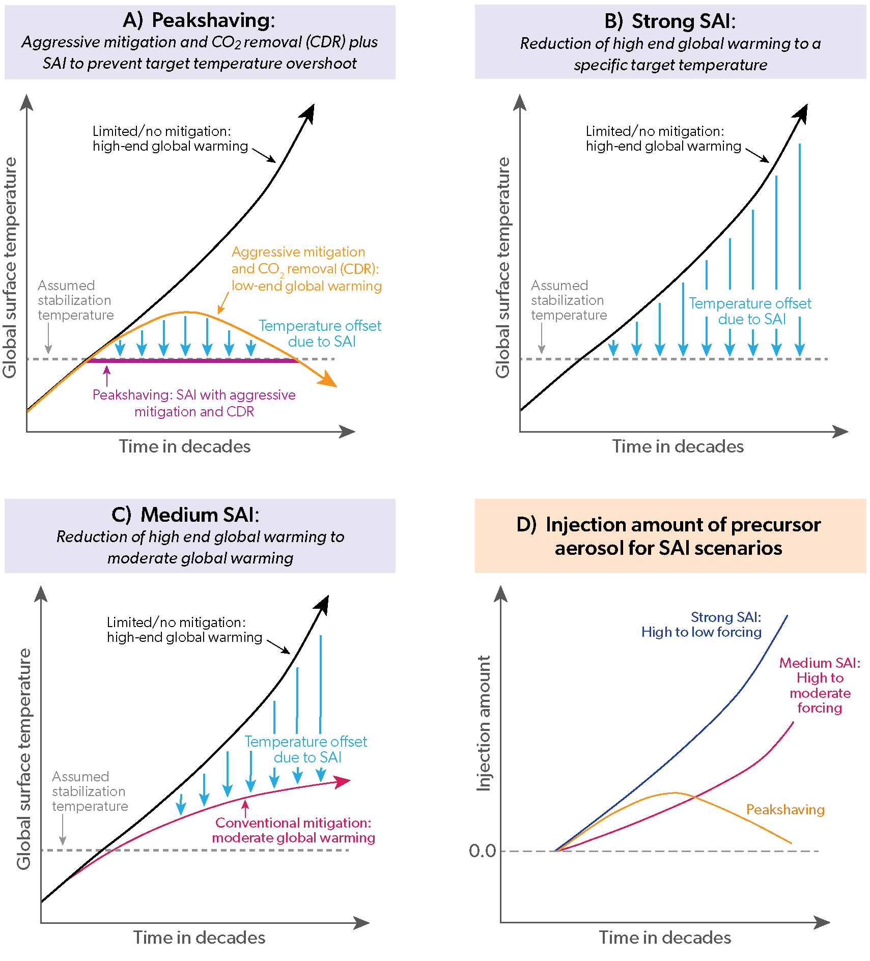
Chapter 7: Scenarios and Information for Policymakers
In its evaluation of future scenarios, this chapter uses reduced complexity models to calculate future impacts on ozone and climate. These models supplement the results from more complex models discussed in Chapters 3-6, with the added advantage that the simpler framework allows exploration of a greater number of scenarios and sensitivity experiments.
Post-Kigali Information of Interest
The Kigali Amendment to the Montreal Protocol, along with regional and national regulatory and voluntary actions taken before Kigali entered into force, is expected to substantially limit future climate forcing by HFCs. Assuming global compliance with the Kigali Amendment, it is expected that HFCs will cause a peak radiative forcing of about 100 mW m-2 by mid-century. This may be compared to some past projections of forcing absent the Kigali Amendment or regulation under another convention, the highest being in excess of 400 mW m-2 in 2050, with substantial increases after that. Given the regional and national regulatory and voluntary actions taken before Kigali entered into force, and assuming global adherence to the Kigali Amendment to the Montreal Protocol, the contribution of HFCs to global annual average warming is projected to be 0.04°C in 2100 (Chapter 2), with a continued decline after that time.
The elimination of all long-lived HFC emissions (including HFC-23) from 2023 onward represents an extreme example of the potential opportunities for future HFC reductions and would reduce the average radiative forcing over 2023-2100 by 79 mW m-2, with additional benefits continuing after 2100. This is more than twice the benefit of eliminating all controlled ODS emissions from the baseline scenario and would reduce the warming attributable to all HFCs to less than 0.01°C by 2100. Of the 79 mW m-2, 51 mW m-2 arises from future production and usage of long-lived HFCs (excluding HFC-23), 16 mW m-2 comes from future emissions from current banks, and 11 mW m-2 comes from emissions of HFC-23.
If emissions of HFC-23, a potent greenhouse gas, remain at the current relative level compared with HCFC-22 production, HFC-23 has the potential to cause about half of the climate forcing (30 mW m-2) of all the other HFCs, combined, by 2100. HFC-23 is emitted into the atmosphere mainly as a by-product from the production of HCFC-22. Its emissions relative to the amounts of HCFC-22 produced have not changed much in recent years and are higher than would be expected if state-of-the-art destruction had been performed during the HCFC-22 production process. While the Kigali Amendment to the Montreal Protocol requires that HFC-23 be "destroyed to the extent practicable," this requirement and the connected reporting of emissions went into effect only on 1 January 2020, and thus reporting is still incomplete and the global response is unclear. Through 2019, the emissions of HFC-23 as a fraction of HCFC-22 production indicate that a considerable part of the produced HFC-23 was still being released unabated into the atmosphere.
Other sources of HFC-23 emissions to the atmosphere may exist and could contribute to its atmospheric burden. There could be contributions to HFC-23 abundances through formation and loss during the production of tetrafluoroethene (TFE) and from the incineration of HCFC-22. Furthermore, direct emissions could grow from the use of HFC-23 in low-temperature refrigerants, although it is not the only refrigerant used in this application.
The Kigali Amendment's control of high-GWP HFCs is expected to lead to overwhelmingly positive climate benefits. Nevertheless, there is a potential for certain negative side effects. Hydrofluoroolefins (HFOs) are increasingly used for replacing high-Global Warming Potential (GWP) HFCs in refrigeration, foam blowing, and various other applications. This replacement leads to less climate change. However, high-volume usage of CCl4 (carbon tetrachloride) as a feedstock in the production of HFOs, a usage and production not controlled by the Montreal Protocol, could lead to sustained elevated abundances of CCl4 if current techniques are continued and some fraction of feedstock production continues to be emitted. A second side effect is that HFO-1234yf emitted into the atmosphere will be fully converted to the stable trifluoroacetic acid (TFA; see below).
Trifluoroacetic acid (TFA), which is produced in the atmosphere from the degradation of HFCs, HCFCs, HFOs, and HCFOs, is not expected to harm the environment over the next few decades, although some regional concerns have been raised; periodic evaluation of this assessment is suggested, as important gaps in our understanding remain. This assessment is based on updated estimates of the TFA formation from current atmospheric concentrations of HFCs and HCFCs (hydrochlorofluorocarbons) and their projected decline, as well as the expected increasing abundance of HFOs as HFC and HCFC replacements within the next years. With long-lived HFCs being replaced with high-TFA-producing, short-lived HFOs, more TFA will be formed in the atmosphere. Because of the shorter lifetime of HFOs, this TFA is expected to be deposited nearer to the location of emissions. Other anthropogenic sources of TFA, such as the incineration of polytetrafluoroethene (PTFE), could also contribute. In view of changing and potential unknown sources, concentrations of TFA should be monitored for changes in different parts of the environment, with a special focus on highly populated regions and on the remote ocean.
Updates on the Climate Impact of Gases Controlled by the Montreal Protocol
In the baseline scenario, future emissions of HFCs (excluding HFC-23), HFC-23, HCFCs, and CFCs contribute approximately 68, 11, 9, and 9 mW m-2 to radiative forcing, respectively, averaged over the 2023-2100 period. Of the 68 mW m-2 from HFCs, 51 mW m-2 arise from future production. For reference, CO2 (carbon dioxide) emissions from fossil fuel usage over this time period are projected to contribute an average of about 3,250 mW m-2 in the SSP2-4.5 scenario. The total radiative forcing from CFCs, HCFCs, and their HFC replacements is projected to continue to remain roughly constant for the next decade or two. After about 2040, the ODS and HFC restrictions of the Montreal Protocol, if adhered to, are expected to ensure a continued decline in the total RF from ODSs and their replacements. Previous expected increases in RF driven by projected HFC increases throughout the century are now mitigated by assumed compliance with the Kigali Amendment.
The effective radiative forcing of the halocarbons has been revised to encompass lower values due to a larger range of estimated negative forcing from the ozone depletion they cause. This offset of the halocarbon direct radiative forcing remains highly uncertain.
Ozone-Depleting Substances (ODSs) and Their Replacements: Impacts on Ozone and Climate
Below, we discuss potential trajectories of equivalent effective stratospheric chlorine (EESC; a proxy for ozone depletion) and radiative forcing (a proxy for climate change) that result from our current understanding of the emissions of individual gases or groups of gases and the processes that lead to these emissions. We reference these potential changes to the so-called baseline scenario, which should be considered a plausible future pathway for these gases that is consistent with the controls of the Montreal Protocol. The specific assumptions made in the baseline scenario can be extremely important to the results. Note that the combined impact of changing assumptions is not always simply the addition of each of the changes. It is also important to recognize that the return date of EESC to 1980 levels is quite sensitive to any change in the EESC concentration because of the relatively small rate at which the EESC is projected to decline around the middle of this century. While a change in the return date to 1980 EESC levels measured in tenths of years or even a few years cannot be discerned in the atmosphere, primarily due to natural variability, this metric can be useful for comparing various alternative ODS scenarios.
It should also be noted that the EESC formalism adopted here is the same one that was applied in Appendix 6C of WMO (2018) and reflects our improved scientific understanding of EESC (see Section 7.3). This alters the time evolution of EESC and dates when EESC returns to 1980 levels when compared with the older approach used in the main part of Chapter 6 of the last Assessment, but it has little effect on the relative impacts of the various alternative future scenarios. If EESC comparisons are made with WMO (2018), it is most appropriate to compare to those found in Appendix 6C rather than Table 6-5 of that Assessment.
Changes in the current baseline scenario lead to a delay in the return of mid-latitude and polar EESC to 1980 levels by 4 years and 7 years, respectively, compared with the baseline scenario in the previous Assessment. This is due mainly to a larger assessed CFC-11 bank, and to a lesser degree, to a larger assessed CFC-12 bank. The larger bank for CFC-11 does not include any explicit increase due to unreported production over the past decade, as that amount is highly uncertain.
The unexpected emissions of CFC-11 declined after 2018. The continued elimination of this emission and the production that has caused it will prevent a substantial impact on ozone and climate. Cumulative unexpected emissions over 2012-2019 have been estimated at 120-440 Gg. Since then, these annual emissions have diminished substantially from their peak amount. The integrated emissions over this period are calculated to lead to a delay in the return of mid-latitude EESC to 1980 levels by about one year and to cause an additional radiative forcing of 2 mW m-2 averaged over 2023-2100. It is unclear how much of the production that led to these emissions has gone into banks, as opposed to having already been emitted. If the unexpected emissions over 2012-2019 were associated with the production of insulating foams, it is estimated that they would have accounted for 25% to 45% of the unreported production, with the rest (146-1320 Gg) going into the CFC-11 bank. The impact of any increase in the bank can be estimated from knowing that a hypothetical 1,000 Gg added to the 2020 bank delays the return of mid-latitude EESC to 1980 levels by almost four years and leads to an additional averaged radiative forcing over 2023-2100 of about 6 mW m-2.
The hypothetical elimination of all future ODS emissions would bring forward the return of mid-latitude and polar EESC to 1980 levels by 16 years and 19 years, respectively, and increase the average of global stratospheric ozone levels in the period 2020-2070 by about 2 DU. It would also reduce average radiative forcing by 31 mW m-2 averaged over 2023-2100. These emissions are dominated by the release from current banks, with a smaller contribution from future production of ODSs that is controlled by the Montreal Protocol and emissions associated with production intended for feedstock purposes. Estimates of bank siz-es are highly uncertain though; the bank approach used in the scenarios here has resulted in substantially larger 2020 banks than estimated in the previous Assessment.
In the baseline scenario, future emissions from current CFC banks contribute more to EESC than do emissions from either HCFC banks or halon banks. However, given the uncertainty in estimates of current bank sizes, these differences are likely not statistically signifi-cant. An elimination of the emissions from the CFC banks are calculated to bring forward the return of mid-latitude EESC to 1980 levels by about 5 years. In this chapter, there is no evaluation made regarding the accessibility of various banks in terms of recapture and destruction.
In the baseline scenario, future emissions from current HCFC banks contribute more to climate change than do future emissions from either CFC banks or halon banks. However, the differences in the climate impacts between the banks of HCFCs and CFCs are likely not statistically significant. Again, there is no evaluation made regarding the accessibility of various banks in terms of recapture and destruction.
Elimination of future emissions of methyl bromide (CH3Br) from quarantine and pre-shipment (QPS) applications, not controlled by the Montreal Protocol, would accelerate the return of mid-latitude and polar EESC to 1980 levels by about two years and would increase globally averaged total ozone by 0.2 DU when averaged over 2020-2070. Production for QPS use has remained relatively stable over the last two decades and now constitutes almost 99% of reported production of CH3Br, since emissions from other uses have declined dramatically. Non-QPS applications of CH3Br were completely phased out in 2015, except for approved critical use exemptions (CUEs). These CUEs have declined by a factor of ~200 since 2005 and make up the remaining ~1% of reported production. CH3Br has little direct impact on climate.
Otherwise-controlled ODSs have increasingly been used as feedstocks. With estimated emission rates of 2-4% (4.3% for CCl4) from the produced ODSs, this has resulted in estimated emissions associated with ODS feedstock applications of 37-59 Gg (15-19 ODP-Gg) in 2019. The influence on ozone of these emissions was dominated by emissions from the feedstock use of CCl4. When compared to the baseline scenario, in which these emissions continue at current levels, an elimination of emissions associated with feedstock use would bring forward the return of mid-latitude and polar EESC to 1980 levels by about 4 and 5 years, respectively. Between 2009 and 2019, the mass of ODSs used as feedstocks, which is not controlled under the Protocol, increased by 75%. When expressed in units of Gg ODP (Gg multiplied by the Ozone Depletion Potential), the increase in feedstock-linked production was only 41% over the same period, as HCFC-22, with a relatively low ODP, was responsible for the highest growth. Eliminating all these emissions in the future would reduce averaged radiative forcing by 6 mW m-2 compared with the baseline scenario.
Of the feedstock production reported, estimated emissions from CCl4 and HCFC production dominate the impact on climate over the coming decades. These two groups lead to an increased average radiative forcing over 2023-2100 of 5 mW m-2 in the baseline scenario. The size of this climate effect is dependent on the assumptions made in the baseline scenario regarding feedstock production growth.
CCl4 feedstock production and usage increased by a factor of about two within the last decade. If CCl4 emissions associated with these allowed uses continue to grow through 2030 as they have been growing over the past decade, future CCl4 atmospheric concentrations will decline more slowly and will be about twice as high (+20 ppt) in 2100 than in the baseline scenario, in which feedstock-related emissions remain constant. As reported in the 2018 Assessment, CCl4 emissions inferred from atmospheric observations continue to be considerably higher than those estimated from feedstock uses, as reported to the United Nations Environment Programme (UNEP), and other known sources. CCl4 emissions related to its feedstock production and usage have been assessed to be 4.3% of the produced amount of CCl4, with a relatively large associated uncertainty. Calculated as ODP-weighted emissions, the emissions from feedstock use of CCl4 in 2019 was 11.2 ODP-Gg yr-1, or 60-74% of all feedstock-related emissions. This is important, as the usage of CCl4 is projected to continue to increase because of its application in the growing production of HFOs in the replacement of the long-lived HFCs. An elimination of all future CCl4 emissions associated with feedstock usage would reduce radiative forcing by about 2 mW m-2 compared with the baseline scenario when averaged over 2023-2100.
In addition to CCl4, the most important contributions to ODP-weighted emissions from other ODSs used as feedstock are from CFC-113 and CFC-114 (2.3-4.6 ODP-Gg), from HCFC-22 (0.5-1.1 ODP-Gg), and from the sum of other HCFCs (0.1-0.3 ODP-Gg), with highest contribution from HCFC-142b. These are based on estimated emissions of 2-4% relative to the production amount. The increased use of HCFC-22 and other HCFCs as feedstocks for fluoropolymer production within the last decades is expected to continue into the future. On the other hand, the usage of feedstock chemicals for the production of HFCs will likely decline because of the Kigali Amendment.
The production and usage of short-lived chlorinated solvents is not controlled by the Montreal Protocol, and some are used in large amounts. Their impact on stratospheric ozone, and their ODPs, vary depending on the season and location of emissions and could grow in the future even as emissions from long-lived ODSs decline. More than 1,600 Gg of CHCl3 (chloroform) are used as feedstock in the production of HCFC-22. emissions from CHCl3 used as a feedstock are comparable to its solvent emissions. CH2Cl2 (dichloromethane), TCE (trichloroethene), and PCE (perchloroethene) are also used as feedstock chemicals, although their emissions are dominated by emissive uses (e.g., from solvents).
Sustained increases in anthropogenic chlorinated very short-lived substance (VSLS) emissions, as seen for CH2Cl2 over the last two decades, would lead to more stratospheric ozone depletion in the future. While observed growth rates of CH2Cl2 have been highly variable and future projections are believed to be highly uncertain, emissions have continued to increase since the last Assessment. If emission rates remain constant at their present level into the future, CH2Cl2 is projected to deplete 0.8-1.7 DU averaged over 2020 to 2070 compared to a case of zero future emissions. Any reduction in the production and consumption of CH2Cl2 would have a rapid impact on ozone, since this VSLS is both emitted soon after production and is cleansed out of the stratosphere within a few years.
A reduction in future N2O emissions from that in the baseline scenario (SSP2-4.5) to that in the SSP scenario with the strongest N2O mitigation (SSP1-1.9) results in a 0.5 DU increase in ozone averaged over 2020 to 2070, or about one-quarter of the impact of eliminating all emissions from controlled ODSs beginning in 2023. This emission reduction also leads to a radiative forcing reduction of 43 mW m-2 averaged over 2023-2100. The magnitude of this N2O reduction represents a decrease in anthropogenic N2O emissions of 3% compared with the baseline scenario when averaged over 2020-2070.
Impacts of Mitigation Options and Particular Scenarios
Figure 7-1 (also shown as Figure ES-8 in this document) shows the ozone and climate-relevant changes that would occur if various actions were to be taken. These changes are shown as the differences in global total column ozone averaged over 2020-2070 and in radiative forcing averaged over 2023-2100, both relative to the baseline scenario, which includes the Kigali Amendment controls for HFCs in Annex F, Group 1. The options available to hasten the recovery of the ozone layer are somewhat limited, mostly because past actions have already been very successful at reducing emissions of ODSs and their replacements.
For the ODSs, the single most effective ozone-depletion and climate change mitigation option, not considering technical feasibility, is bank recapture and destruction of the CFC banks; however, large uncertainties in the CFC-11 and CFC-12 banks have been reported in the literature, with the recent production associated with the unexpected emissions of CFC-11 further adding to uncertainties in the bank sizes. Furthermore, no assessment has been made here regarding the fraction of the banks that are accessible for capture or the fraction that are active.
For CH3Br, elimination of production for currently uncontrolled QPS applications is shown.
For CCl4, the impact of eliminating emissions from controlled production starting in 2023 is shown.
For CH2Cl2, an uncontrolled ozone-depleting gas with an atmospheric lifetime of ~180 days, future emissions continue to have the potential to lead to more ozone depletion than emissions from many of the other alternative scenarios explored here. CH2Cl2 is emitted mainly from Asia, and emissions and concentrations have been growing steadily in recent years.
For N2O, the impacts of a strong mitigation scenario (SSP1-1.9) are compared to the baseline scenario (SSP2-4.5).
For HFCs, the impact of a hypothetical complete global phaseout of production (excluding HFC-23) starting in 2023 is shown. An additional scenario is included in which HFC-23 emissions are reduced to virtually zero, consistent with the current best practice of incineration, rather than the assumed emissions rate of 1.6% of HCFC-22 production included in the baseline scenario, in order to show the effect of nearly eliminating by-product emissions.
Updates on Impacts of Greenhouse Gases and Other Processes on Future Stratospheric Ozone
In this section, we summarize potentially important impacts on the future of the ozone layer that could result from anthropogenic activity not associated with ODS or replacement production and consumption and thus that is not controlled by the Montreal Protocol. Net stratospheric cooling, which is projected in many scenarios due to increases in greenhouse gas concentrations, is predicted to lead to increases in upper-stratospheric ozone at all latitudes, with a more complex pattern of ozone changes in the lower stratosphere, including a decrease at tropical latitudes driven by changes in dynamics and transport; these processes are discussed in detail in Chapters 3 and 4. Potential climate intervention activities that may affect ozone are discussed in Chapter 6.
Our ability to accurately predict future changes in the ozone layer continues to be limited more by uncertainties in the future levels of CO2, CH4 (methane), and N2O than by uncertainties in the levels of ODSs. Global mean tropospheric warming, as well as stratospheric cooling, will drive ozone changes through both atmospheric circulation and chemistry, while changing CH4 and N2O will lead to further changes in the chemistry associated with stratospheric ozone. Future ozone levels depend on the path of greenhouse gas emissions and aerosol abundances, as well as the sensitivity of the climate system to these emissions.
Rocket launches presently have a small effect on total stratospheric ozone (much less than 0.1%). However, rocket systems using new propellants (e.g., hydrogen and methane) could exert a substantial influence in the future. The future scenarios of space industry emissions consider the potential for a significant increase in launch rates, the adoption of new launch-vehicle propellants, and an increase in middle-atmosphere aerosol and the production of NO (nitrogen monoxide) by reentering space debris. Many of the impacts of rocket activity involve chemistry and radiative interactions that are poorly understood and, in some cases, not yet studied. Furthermore, the planned development of massive low-Earth orbit satellite constellations (megaconstellations) could cause particulates resulting from space debris reentry to become comparable to that from launch emissions; little is known about the impacts of reentry particles, and their accumulation in the stratosphere has not been modeled. The uncertainties in these processes and in any potential new emission sources limit the confidence level of predictions of present and future impacts of space industry emissions on stratospheric ozone. Periodic assessment and critical knowledge gap identification are warranted.
The influence of hydrogen as an energy carrier on stratospheric ozone remains uncertain. Hydrogen-based energy will likely play a role in a future non- or reduced-fossil economy. However, if it is not a dominant energy carrier, it is unlikely that it will significantly affect ozone. This statement should be re-evaluated periodically.
The impacts of supersonic aircraft on stratospheric ozone are discussed in Chapter 4.
Climate intervention approaches that affect the stratospheric ozone layer are discussed in Chapter 6.
Footnotes
- Decision XXXI/2: Potential areas of focus for the 2022 quadrennial reports of the Scientific Assessment Panel, the Environmental Effects Assessment Panel and the Technology and Economic Assessment Panel
- Montreal Protocol Handbook, 2018.
- Uncertainties in absolute changes of atmospheric abundances were derived using the 1 standard deviation measurement uncertainties (where appropriate combined as the square root of the sum of their squares) and the bootstrap algorithm described in Barreto and Howland (2006). Similar to the procedure described in Leedham Elvidge et al. (2018), and to represent atmospheric variability, data was converted to a dataset comprised of 1) original data, 2) original data minus measurement uncertainty and 3) original data plus measurement uncertainty. This dataset was then resampled (with replacement) 1000 times to derive a standard deviation that is a realistic representation of the uncertainty of the entirety of the original data.
- The global zonal mean circulation that transports mass, heat, and tracers in the stratosphere.
- Based on an adapted SSW definition in the Southern Hemisphere; see Section 5.2.6.1.
- Quasi-periodic (period ~28 months) oscillation of stratospheric equatorial winds from easterly to westerly.
- Arctic amplification refers to the ratio of Arctic warming (60-90°N) to global warming over a given time period.